Sensitivity study: differentiable pipeline, scale cuts and degeneracy breaking

This page answers one question, pedagogically:

How much cosmological information sits at small scales, and under what condition can we actually use it?

The short answer, demonstrated below with the full ZM15 + X-ray gas + AGN pipeline: the sensitivity to the cosmological parameters \((\Omega_m, \sigma_8)\) increases towards small scales, but for clustering and lensing alone that gain is throttled by degeneracies with the galaxy–halo connection. Adding an X-ray and/or a thermal-SZ cross-statistic breaks those degeneracies, which is what lets the small-scale information convert into cosmological constraining power.

Everything here is exact autodifferentiation. The one ingredient that makes that possible is using the analytic Eisenstein & Hu (1998) transfer function for the linear \(P(k)\) instead of CAMB (which is not JAX-traceable): the whole forward model — cosmology included — is then a single differentiable JAX function, and the Fisher Jacobian \(\partial d/\partial\theta\) is one jax.jacfwd call.

Code: hod_mod.forecast (forward model + Fisher engine), hod_mod.scripts.forecasts.run_sensitivity_study (the study), hod_mod.scripts.forecasts.make_sensitivity_figures (these figures).

---

The fiducial model and the twelve summary statistics

We fix a single representative sample — a BGS \(M_*>10\) threshold sample at \(z\simeq0.2\) — at the best-fit parameters of the campaign:

• cosmology — Planck 2018 (\(\Omega_m=0.31\), \(\sigma_8=0.811\); \(h, \Omega_b, n_s\) are free but carry their Planck/BBN priors — they are near-flat directions for these low-\(z\), small-scale probes on their own);

• HOD — the Zu & Mandelbaum 2015 MAP of the BGS joint fit (9 free parameters);

• X-ray gas / AGN — the S1 energy-band MAP (\(L_X\)–\(M\), \(kT\)–\(M\), profile shape p2/r_max, duty cycle log10DC);

• hot-gas / baryon-feedback sector — a mass fraction \(f_b(M)\) and gas puffiness \(\eta(M)\) (parameters log10_M_pivot, log10_eta_min), shared between the lensing, X-ray and tSZ legs (see the baryon section below).

The Fisher vector has 31 parameters: 5 cosmological (\(\Omega_m,\sigma_8,h,n_s,\Omega_b\)), 9 HOD, 6 X-ray gas (\(L_X\)/\(kT\)/profile), 2 baryon-feedback, \(\beta_P\), \(\log_{10}\rm DC\), and 7 for the Powell (2022) AGN X-ray luminosity-function sector (the \(M_{\rm BH}\)–\(M_*\) relation \(\mu_{\rm BH},\alpha_{\rm BH},\sigma_{\rm BH}\), the universal Eddington-ratio distribution \(\log_{10}\lambda_*,\delta_1,\delta_2\), and the active fraction \(\log_{10}f_{\rm ERDF}\)).

From it we predict twelve data vectors: projected clustering \(w_p(r_p)\), galaxy–galaxy lensing \(\Delta\Sigma(R)\), the angular cross/auto power spectra \(C_\ell^{gX}\) (galaxy × X-ray), \(C_\ell^{gy}\) (galaxy × tSZ) and \(C_\ell^{XX}\) (X-ray auto), the cosmic-shear convergence spectrum \(C_\ell^{\kappa\kappa}\) (source \(n(z)\) at \(z_s\simeq0.8\)), three CMB-lensing spectra \(C_\ell^{\kappa_c\kappa_c}\) (auto), \(C_\ell^{g\kappa_c}\) (galaxy×CMB-lensing) and \(C_\ell^{\kappa\kappa_c}\) (shear×CMB-lensing, source at \(z_*\simeq1089\)), the galaxy number density \(n_{\rm gal}\) and stellar-mass function \(\Phi(M_*)\), and the AGN X-ray luminosity function \(\Phi(L_X)\) (an abundance, no length scale — see the AGN section). A constant relative error \(f\) (0.1 %, 1 %, 5 %) is assigned to every data point, so the diagonal covariance is \(C=\mathrm{diag}\!\big((f d_i)^2\big)\); an analytic Gaussian covariance with cross-observable correlations is available as an option (see hod_mod.forecast.covariance).

The derivative of the pipeline, step by step

Because the model is one differentiable function, we can watch a response propagate through it by the chain rule. The figure below shows the logarithmic sensitivity \(\partial\ln O/\partial\ln p\) of each pipeline stage to all five cosmological parameters (\(\Omega_m,\sigma_8,h,n_s,\Omega_b\)), from the linear power spectrum all the way to the observables.

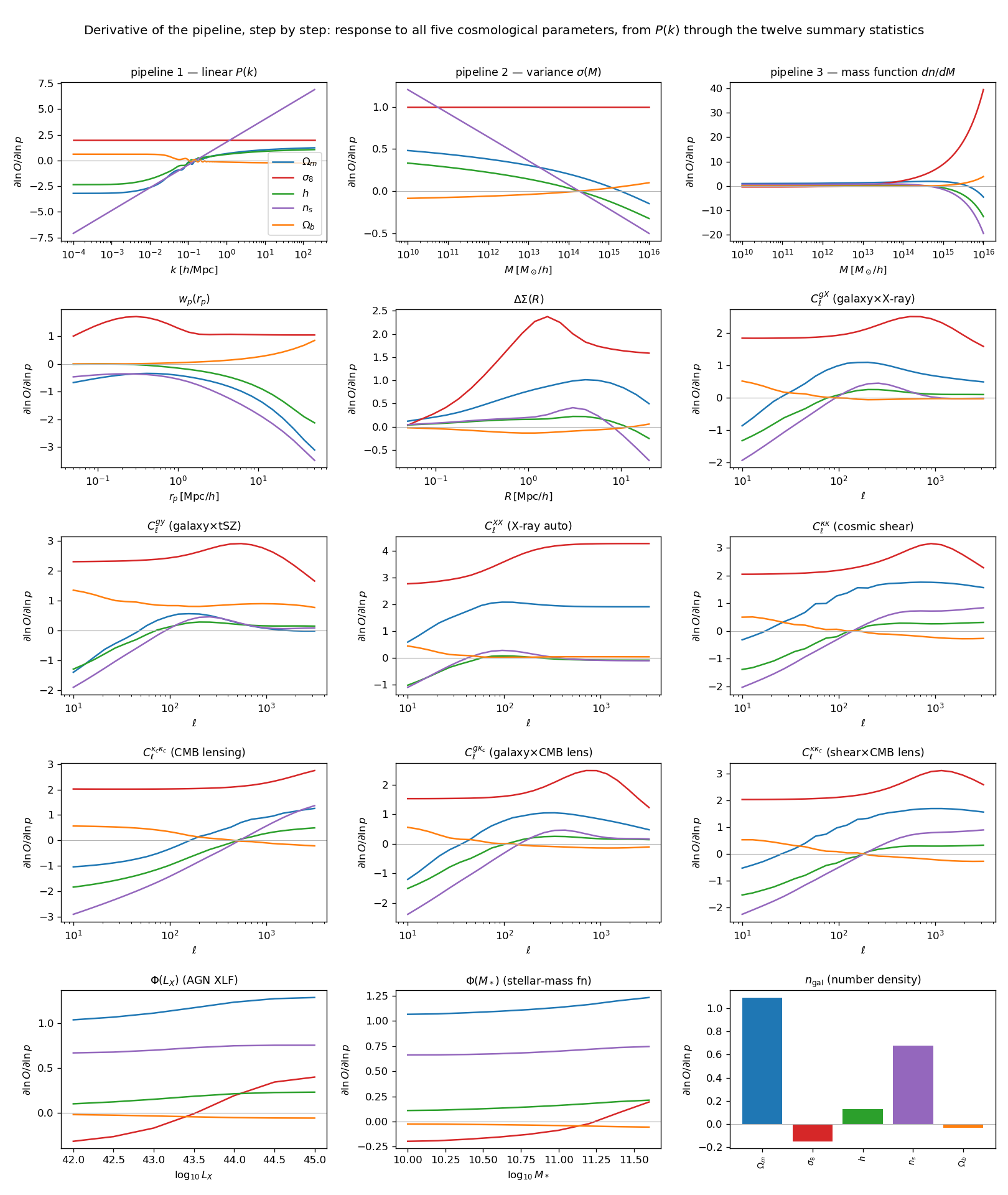
The cosmological derivative propagating through the pipeline (all via JAX autodiff). The first row is the three shared upstream stages: the two exact analytic checkpoints that validate the autodiff — \(\partial\ln P/\partial\ln\sigma_8=2\) everywhere (linear \(P(k)\)) and \(\partial\ln\sigma(M)/\partial\ln\sigma_8=1\) — and the mass function, which shows the hallmark exponential sensitivity at cluster masses (\(\partial\ln(dn/dM)/\partial\ln\sigma_8\to+40\) at \(10^{16}\,M_\odot/h\)), the physical reason massive halos are such sharp cosmological probes. The remaining twelve panels are the endpoint response of every summary statistic — \(w_p\), \(\Delta\Sigma\), the four \(C_\ell\) gas/lensing cross/auto spectra, the three CMB-lensing spectra, the AGN XLF \(\Phi(L_X)\), the stellar-mass function and \(n_{\rm gal}\) — to \(\Omega_m\) (blue) and \(\sigma_8\) (red). The abundances (XLF, SMF, \(n_{\rm gal}\)) inherit the steep mass-function response; the \(C_\ell\) grow towards high \(\ell\). That steep, mass-localised upstream response is exactly what the X-ray, SZ and abundance statistics tap into.

Two things are worth reading off this cascade:

• \(\sigma_8\) enters as a pure amplitude upstream (\(\partial\ln P/\partial\ln\sigma_8=2\)) but its imprint on the observables becomes scale- and mass-dependent downstream, because the halo model reweights it by the mass function and the occupation.

• \(\Omega_m\) changes the shape of \(P(k)\) (panel 1, with the BAO wiggles visible) and the growth, so its response is scale-dependent from the start.

Where the information lives: response functions

The rows of the Jacobian, \(\partial\ln O/\partial\ln\theta\) as a function of scale, are the raw material of the Fisher matrix. They show where on each observable a parameter leaves its mark.

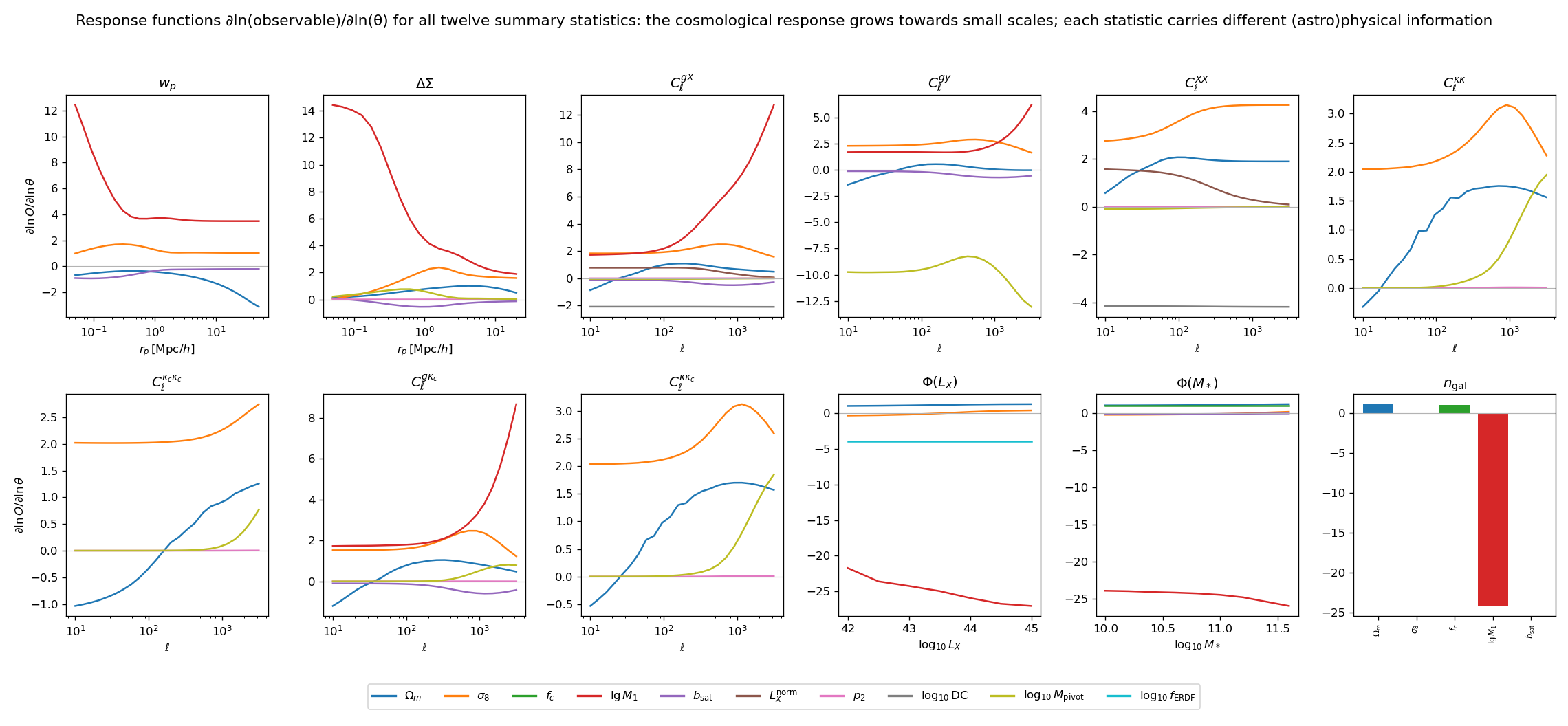
Response functions \(\partial\ln O/\partial\ln\theta\) for all twelve summary statistics (two rows), for a representative set of parameters (legend). The cosmological response (\(\Omega_m,\sigma_8\)) grows towards small scales / high \(\ell\) — there is genuinely more cosmological signal there. But the same small scales are where the astrophysical parameters live: the satellite amplitude \(b_{\rm sat}\) and SHMR shape in \(w_p\)/\(\Delta\Sigma\), the gas parameters (\(L_X\), p2, log10DC) in \(C_\ell^{gX}\)/\(C_\ell^{XX}\), the feedback pivot in \(C_\ell^{gy}\), the active fraction \(f_{\rm ERDF}\) (flat) in \(\Phi(L_X)\), and \(f_c\) in \(n_{\rm gal}\). Note that \(w_p\), \(\Delta\Sigma\), \(C_\ell^{gy}\) and the lensing spectra are blind to the gas/AGN emission parameters, while \(C_\ell^{gX}\)/\(C_\ell^{XX}\)/\(\Phi(L_X)\) carry them — this complementarity is the key to the degeneracy breaking below.

The Fisher matrix and a useful identity

With a constant relative error the Fisher matrix is

\[F_{ab} = \sum_i \frac{1}{(f\, d_i)^2} \frac{\partial d_i}{\partial\theta_a} \frac{\partial d_i}{\partial\theta_b} = \frac{1}{f^{2}}\sum_i \frac{\partial\ln d_i}{\partial\theta_a} \frac{\partial\ln d_i}{\partial\theta_b},\]

where \(f\) is the relative error level (0.1 %, 1 %, 5 %) applied to every data point \(d_i\) — not to be confused with the HOD central completeness parameter \(f_c\) (one of the \(\theta_a\), discussed just below): the scalar \(f\) sets the noise, whereas \(f_c\) is a model parameter being constrained. From the second form, the degeneracy directions do not depend on \(f\) — only the overall size of the error bars scales as \(f\). Parameter constraints follow from \(\mathrm{cov}=F^{-1}\) (with Planck priors optionally added as \(\mathrm{diag}(1/\sigma_{\rm prior}^2)\)). The central completeness \(f_c\) cancels out of \(w_p\) and \(\Delta\Sigma\) exactly, so those probes cannot constrain it; the galaxy number density \(n_{\rm gal}\) (\(\propto f_c\)), which is in this data vector, pins it to \(\sigma/|\theta|\simeq1.8\%\) — and correspondingly \(f_c\) shows a moderate cosmology degeneracy (\(\mathrm{corr}(\sigma_8)=+0.44\)).

Breaking the degeneracies with X-ray and SZ

At small scales the clustering and lensing signals are strongly degenerate with the galaxy–halo connection: a change in \(\sigma_8\) can be mimicked by adjusting the satellite occupation or the scatter of the stellar-to-halo mass relation. The X-ray and SZ cross-statistics see the same halos through their gas and pressure — with a steep, well-localised mass dependence (recall the mass function panel above) — so they pin the occupation and the halo-mass scale independently, and the cosmology↔nuisance degeneracy opens up.

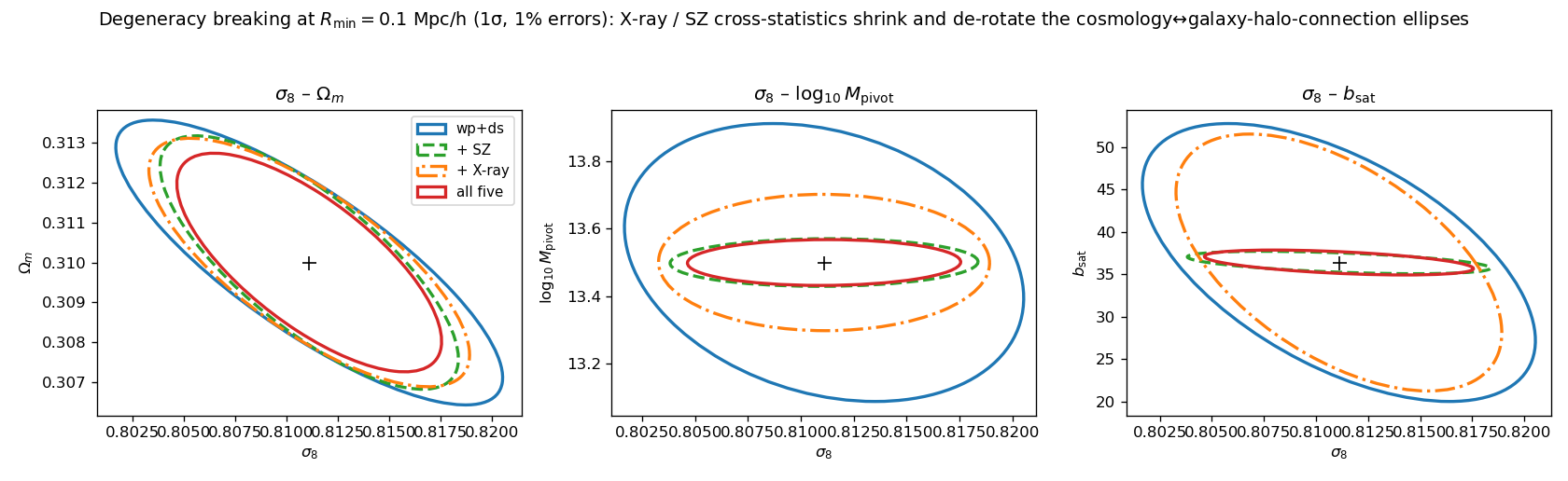
1σ Fisher ellipses at a small-scale cut (\(R_{\min}=0.1\) Mpc/h, 1 % errors, weakly-informative nuisance priors). Adding SZ (green), X-ray (orange) and both (red) shrinks and de-rotates the ellipses of \(\sigma_8\) with \(\Omega_m\), with the baryon-feedback mass scale \(\log_{10}M_{\rm pivot}\) (middle — see the next section), and with the satellite amplitude \(b_{\rm sat}\). De-rotation is the signature of a broken degeneracy, not merely more data.

The result: small scales help — conditionally

Putting it together: we marginalise over the full parameter set (HOD + gas + AGN) and track \(\sigma(\sigma_8)\) and \(\sigma(\Omega_m)\) as the scale cut \(R_{\min}\) is lowered from 10 to 0.1 Mpc/h, for a data vector grown cumulatively to all twelve summary statistics.

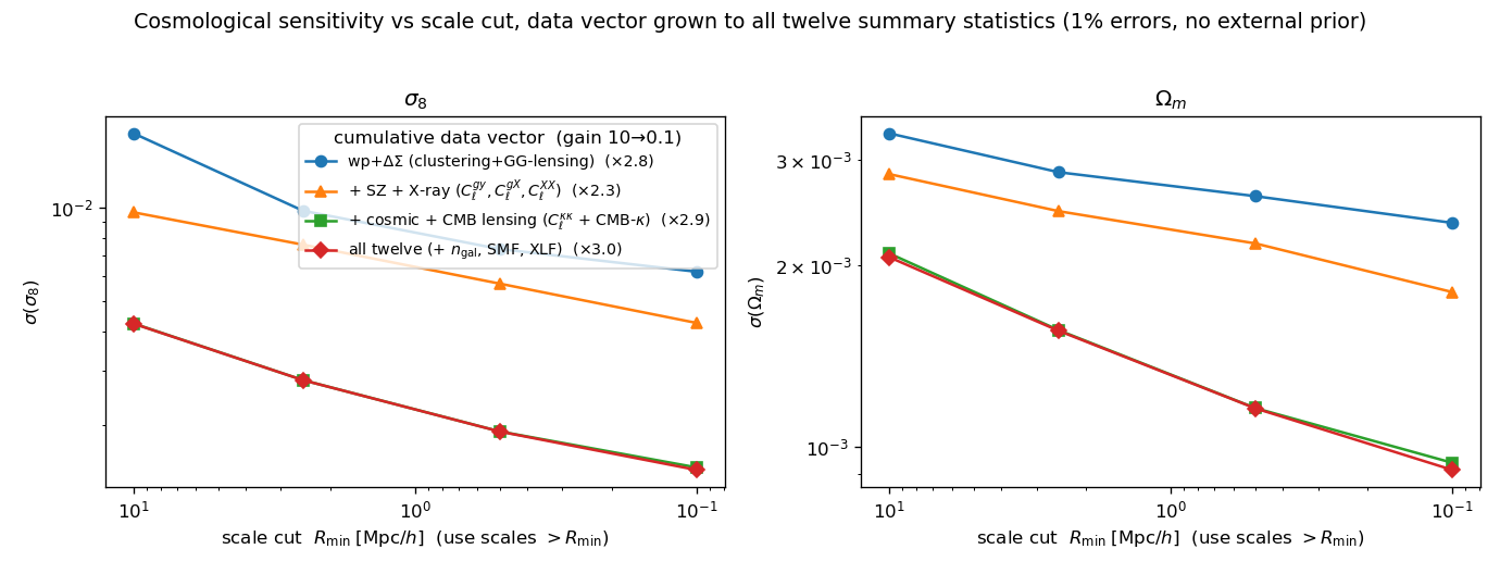
Small scales to the right; 1 % errors, no external prior. The data vector grows cumulatively: clustering + galaxy–galaxy lensing (blue), \(+\) SZ \(+\) X-ray (orange), \(+\) cosmic shear and the CMB-lensing triplet (green), and finally all twelve summary statistics (red, adding \(n_{\rm gal}\), the SMF and the AGN XLF). Every set tightens by a similar \(\times2\text{–}3\) from \(R_{\min}=10\) to \(0.1\) Mpc/h (for \(\sigma_8\): \(\times2.8\), \(\times2.3\), \(\times2.9\), \(\times3.0\)); the payoff is in the absolute level. Two features stand out. (i) The lensing spectra dominate the gain — adding cosmic shear + CMB lensing drops \(\sigma(\sigma_8)\) at \(R_{\min}=0.1\) Mpc/h from \(4.3\times10^{-3}\) (\(+\)SZ+X-ray) to \(1.5\times10^{-3}\), and \(\sigma(\Omega_m)\) from \(1.8\times10^{-3}\) to \(9.4\times10^{-4}\). (ii) Abundance adds almost nothing to the cosmology (red overlaps green): \(n_{\rm gal}\), the SMF and the XLF constrain \(f_c\) and the SHMR, not \(\sigma_8/\Omega_m\). End to end the full data vector reaches \(\sigma(\sigma_8)=1.4\times10^{-3}\) and \(\sigma(\Omega_m)=9.2\times10^{-4}\) — a factor \(\times4.3\) and \(\times2.6\) below clustering+lensing alone.

The physical reading:

• Large scales (two-halo, linear): all probes measure essentially the same thing (\(b_{\rm eff}^2 P_{\rm lin}\)), so extra statistics add little and the cosmology error is prior/limited.

• Small scales (one-halo): more cosmological signal is present, but for galaxies alone it is entangled with the occupation. The X-ray and tSZ cross-correlations supply an independent handle on the halo occupation and mass scale, so the small-scale cosmological information becomes usable.

In other words, the small-scale cosmological sensitivity is real but latent: the gas (X-ray/tSZ) cross-statistics unlock it for the galaxy probes, while the lensing power spectra — cosmic shear and CMB lensing — contribute the largest independent share of the total gain. The abundance statistics (\(n_{\rm gal}\), SMF, XLF) instead target the occupation (\(f_c\), the SHMR), leaving \(\sigma_8/\Omega_m\) essentially unchanged.

Baryonic feedback: contaminating lensing, calibrated by X-ray / SZ

The strongest version of the argument involves baryons directly. Feedback (AGN + stellar) expels hot gas from group-scale halos, redistributing a mass fraction \(f_b(M)\) from the compact dark-matter cusp into an extended hot atmosphere. That redistribution modulates the small-scale matter distribution probed by lensing — and it is the same hot gas that emits the X-rays and sources the tSZ pressure. We add this as a single shared hot-gas sector to the model: a mass fraction \(f_b(M)\) (a sigmoid with feedback-mass-scale \(\log_{10}M_{\rm pivot}\); BaryonFractionSigmoid) follows an extended gas profile (puffiness \(\log_{10}\eta_{\min}\), truncated at \(r_{\max}R_{200}\)). These two parameters enter ΔΣ (the CDM+gas split, an exact port of delta_sigma_split()), the X-ray emissivity (\(\propto f_b^2\)) and the tSZ pressure (\(\propto f_b\)) simultaneously.

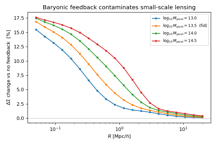
The imprint of feedback on galaxy–galaxy lensing: fractional change in \(\Delta\Sigma(R)\) relative to a no-feedback (cosmic-gas) reference, for several feedback strengths. It is a scale-dependent, few-to-~17 % effect concentrated at \(R\lesssim1\) Mpc/h and it depends on the (a priori unknown) feedback parameters — so it must be marginalised over, and it eats into the small-scale cosmological information.

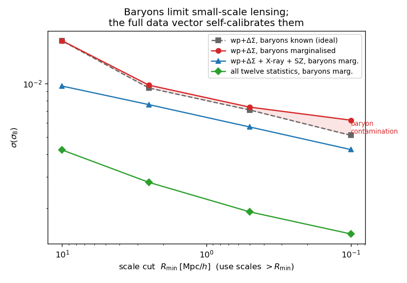
Marginalising over the baryon parameters (red) inflates \(\sigma(\sigma_8)\) above the baryons-known ideal (grey) — the shaded baryon-contamination band, which widens towards small scales. Adding the X-ray and tSZ statistics (blue), which measure the same gas directly, calibrates the baryons and recovers the ideal: at \(R_{\min}=0.1\) Mpc/h baryon marginalisation degrades \(\sigma(\sigma_8)\) by ×1.22 (\(5.1\to6.2\times10^{-3}\)) and adding X-ray/SZ recovers it by ×1.46 (to \(4.3\times10^{-3}\) — below the baryons-known ideal, because the cross-spectra also add their own cosmological information). With the full twelve-statistic data vector (green) the calibration is complete: \(\sigma(\sigma_8)\) reaches \(1.4\times10^{-3}\) (a further \(\times3.6\) below the wp+ΔΣ ideal, driven by the lensing spectra), and marginalising over the baryon parameters now costs only \(\times1.01\) (\(1.423\to1.435\times10^{-3}\)) — the contamination band has effectively closed: the hot gas is self-calibrated by the data.

This closes the loop: baryonic feedback is a genuine small-scale systematic for weak lensing, degenerate with \(\sigma_8\); the X-ray and SZ cross-statistics are direct, high-signal probes of exactly that gas, so combining them removes the systematic and lets small-scale lensing deliver cosmology. For this \(M_*>10\) galaxy–galaxy-lensing sample the contamination is bounded by the group-scale gas fraction (a ~22 % effect on \(\sigma_8\)); it is larger for cosmic shear, treated next.

Cosmic shear: the matter power and where baryons bite hardest

The cosmic-shear convergence spectrum \(C_\ell^{\kappa\kappa}\) — the projected matter power \(P_{mm}(k)\) weighted by the weak-lensing efficiency of a background source population. We build \(P_{mm}\) from the halo model (1-halo with the same baryon-split matter profile, plus the linear 2-halo term) so the identical hot-gas sector that suppresses \(\Delta\Sigma\) also suppresses the shear signal, and project it with the lensing kernel \(W_\kappa(\chi)\) for sources at \(z_s\simeq0.8\).

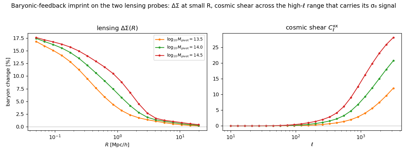
The baryon imprint on the two lensing probes. In \(\Delta\Sigma\) it is confined to \(R\lesssim1\) Mpc/h (often scale-cut away); in cosmic shear it grows monotonically across \(\ell\gtrsim300\)–\(3000\) — exactly the multipoles that carry the shear \(\sigma_8\) signal — reaching \(\sim10\text{–}30\%\) for plausible feedback strengths. Because it cannot simply be cut out, baryon calibration is even more important for shear.

Cosmic shear is a useful \(\sigma_8\) probe: adding it to clustering+lensing tightens \(\sigma(\sigma_8)\) from \(6.2\times10^{-3}\) to \(4.2\times10^{-3}\) (a factor \(\times1.5\), 1 % errors, no external prior). In this regime the marginalised baryon degradation of \(\sigma_8\) is small (\(\sim5\%\)), because the broad \(\ell\) range plus the weakly-informative priors already pin the suppression — but the systematic is real and, at the accuracy of Stage-IV shear, the X-ray/tSZ calibration developed above is exactly what keeps it under control.

Closing the baryon budget energetically

The baryon fraction is below cosmic because feedback has displaced the missing gas. Is there enough energy? We compare, per halo, the energy to unbind the missing baryons, \(E_{\rm disp}=\Delta f_b\,M\,v_{200}^2\), against two feedback channels: AGN, tied to the measured X-ray sector (\(E_{\rm AGN}\propto \varepsilon_{\rm couple}\,10^{\log_{10}\rm DC}\, L_X^{\rm on}(M)\,t_H\), the same duty cycle that sets \(C_\ell^{gX/XX}\)), and stellar/SN (\(E_{\rm SN}\propto M_*(M)\), ZM15 SHMR).

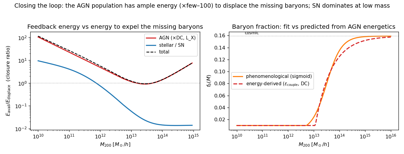
Left: the closure ratio \(E_{\rm avail}/E_{\rm disp}\). The AGN channel (red) exceeds unity at all masses and dips to :math:`approx1` exactly at the group scale (\(\sim2\text{–}3\times10^{13}\,M_\odot/h\)) where expulsion is hardest — a self-regulation signature — needing only \(\varepsilon\sim1\%\) mechanical coupling of \(M_{\rm BH}c^2\) (or of the bolometric AGN output). The stellar/SN channel (blue) suffices only below \(\sim10^{12}\,M_\odot/h\), the natural low-mass regime. Right: the baryon fraction predicted from this energy balance tracks the phenomenological fit.

Two conclusions. (i) The loop closes: the simulated AGN population carries ample energy (a factor few–100 surplus) to displace and heat the missing baryons, with stellar feedback taking over at dwarf scales — so the sub-cosmic baryon fractions are energetically consistent. (ii) Closure ≠ constraining power (yet): replacing the phenomenological baryon parameter with the physical coupling \(\varepsilon_{\rm couple}\) is a one-for-one trade, so \(\sigma(\sigma_8)\) is essentially unchanged — even when \(\varepsilon_{\rm couple}\) is tied to the X-ray-constrained duty cycle, because cosmic shear already pins \(\sigma_8\). The energy model’s value is physical: it turns \(f_b(M)\) from a free nuisance into a prediction of the (observed) AGN + stellar populations. Genuine statistical gain would follow from folding in the measured AGN X-ray luminosity function and \(M_{\rm BH}\) census as data, so the feedback normalisation is pinned externally rather than fitted — the natural next step. This mode is available as ForwardModel(energy_closure=True).

The AGN X-ray luminosity function as a cosmology probe

The energy section ended on a promise: fold in the measured AGN X-ray luminosity function so the accretion sector is pinned by data rather than fitted. We now do exactly that, with the physical Powell (2022) AGN–halo model (hod_mod.agn.powell.PowellAGNModel, validated standalone against the Aird+2015 hard XLF). It forward-models the SMBH luminosity per halo — the ZM15 SHMR gives \(\langle\log M_*\rangle(M_h)\); a free \(M_{\rm BH}\)–\(M_*\) relation gives \(\langle\log M_{\rm BH}\rangle\); a universal Eddington-ratio distribution (Ananna 2022 broken power law) sets the accretion; \(L_{\rm bol}=1.26\times10^{38}\,M_{\rm BH}\lambda\) — and integrates it over the halo mass function:

\[\Phi(\log L_X) = f_{\rm ERDF}\!\int\! \mathrm d\log M_h\; \frac{\mathrm dn}{\mathrm d\log M_h}(\Omega_m,\sigma_8)\; P(\log L_X\,|\,M_h).\]

Because the amplitude and shape of \(\Phi\) carry \(dn/dM_h\), the XLF is — like the cluster mass function — a cosmological probe; and its shape simultaneously pins the AGN sector that contaminates \(C_\ell^{gX}\)/ \(C_\ell^{XX}\). It is one of the twelve observables, fully differentiable (a shift-invariant ERDF⊛Gaussian kernel), so the single jax.jacfwd also returns \(\partial\Phi/\partial\theta\).

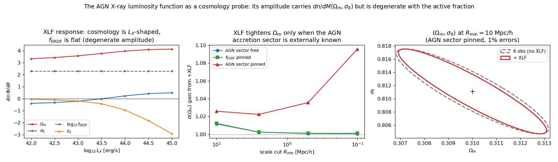
Left: the XLF response \(\partial\ln\Phi/\partial\theta\). The cosmological response is large but \(L_X\)-dependent (\(\partial\ln\Phi/\partial\Omega_m\simeq+3.3\to+4.1\) rising with \(L_X\), and \(\sigma_8\) even rotates sign across \(L_X\)), whereas the active fraction \(f_{\rm ERDF}\) is a flat amplitude (\(\partial\ln\Phi/\partial\log_{10}f_{\rm ERDF}=\ln 10\), grey dashed): the XLF’s cosmological amplitude is therefore degenerate with \(f_{\rm ERDF}\), and only its shape is uniquely cosmological. Middle: the resulting \(\sigma(\Omega_m)\) improvement from adding the XLF, versus scale cut, under three external-knowledge scenarios of the AGN accretion sector. Right: the \((\Omega_m,\sigma_8)\) ellipse at \(R_{\min}=10\) Mpc/h with (red) vs without (grey) the XLF when the AGN sector is externally pinned.

The result is clean and physical (1 % errors, no Planck prior):

• AGN sector marginalised (free): the XLF adds essentially nothing to \((\Omega_m,\sigma_8)\) (\(\lesssim1\%\)). Its cosmological signal is amplitude-dominated, and that amplitude is soaked up by the unknown active fraction \(f_{\rm ERDF}\) — exactly the flat degeneracy direction in the left panel.

• Active fraction externally known (\(f_{\rm ERDF}\) pinned alone): still \(\lesssim1\%\) on \(\sigma(\Omega_m,\sigma_8)\) — pinning the amplitude is not enough while the ERDF shape floats.

• Full AGN sector pinned (local \(M_{\rm BH}\)–\(M_*\) + Eddington-ratio census): the XLF tightens the \((\Omega_m,\sigma_8)\) figure of merit by ×1.20 at \(R_{\min}=10\) Mpc/h (with \(\sigma(\Omega_m)\) ×1.03 there), and \(\sigma(\Omega_m)\) by ×1.10, \(\sigma(\sigma_8)\) by ×1.09 at \(R_{\min}=0.1\) Mpc/h.

The lesson mirrors the baryon story, one level deeper: the AGN luminosity function does carry cosmology, but latently — its constraining power is unlocked not by a scale cut but by external knowledge of the accretion physics (the \(M_{\rm BH}\) census and Eddington-ratio distribution). Even then, in this twelve-observable combination the gain is modest (~10–20 % on the \((\Omega_m,\sigma_8)\) FoM), because the abundance information the XLF adds is largely already supplied by the other probes (\(n_{\rm gal}\), the SMF, cosmic shear and CMB lensing) — the concrete realisation of the “fold in the XLF and the \(M_{\rm BH}\) census” step promised above.

Parameter inventory: what carries cosmological vs astrophysical information

The forecast has 31 parameters. Being exhaustive about their information content is the whole point: five are cosmological (two targets plus three Planck/BBN-calibrated), and the other 26 are astrophysical — but they are not all equal. Some astrophysical parameters are degenerate with cosmology (marginalising over them inflates \(\sigma(\Omega_m,\sigma_8)\), and they are exactly what the X-ray/SZ/XLF statistics calibrate); others are cleanly separated (they carry only astrophysics and marginalising over them barely touches cosmology). The classification below is read directly off the Fisher matrix (marginalised \(\sigma\), the probe that supplies each parameter’s information, and the correlation with \(\Omega_m,\sigma_8\)), at the reference configuration \(R_{\min}=0.1\) Mpc/h, 1 % errors, no Planck prior on the targets (\(h,n_s,\Omega_b\) carry their Planck/BBN priors).

1. Cosmological parameters (5). The two targets are \(\Omega_m\) (\(\sigma/\theta\approx0.30\%\)) and \(\sigma_8\) (\(0.18\%\)), spread across the amplitude-sensitive statistics — the X-ray auto \(C_\ell^{XX}\), cosmic shear \(C_\ell^{\kappa\kappa}\), CMB lensing, the cross-spectra and \(w_p\) — and mutually correlated at \(-0.89\). The three calibrated parameters \(h\) (\(0.6\%\)), \(n_s\) (\(0.3\%\)) and \(\Omega_b\) (\(0.9\%\)) still carry their Planck/BBN priors, but with cosmic shear and CMB lensing now in the vector they are no longer purely prior-held: CMB lensing and \(w_p\) tighten \(h\) below its Planck width (\(0.8\%\to0.6\%\)) and similarly for \(n_s\), while \(\Omega_b\) is measured mostly by the tSZ \(C_\ell^{gy}\) (whose pressure scales as \(\Omega_b/\Omega_m\)), improving on BBN alone. They remain near-flat directions for cosmology, correlated with the targets only at \(|\mathrm{corr}|\lesssim0.35\).

2. Astrophysical nuisances that are degenerate with cosmology (7) — the ones that must be marginalised or externally calibrated:

• \(\log_{10}\rm DC\) (X-ray duty cycle) — the strongest cosmology degeneracy, \(\mathrm{corr}(\sigma_8)=-0.44\): it is a pure amplitude on \(C_\ell^{XX}\)/\(C_\ell^{gX}\), exactly where \(\sigma_8\) also sits. Very tightly measured (\(0.14\%\)) because it shares that amplitude.

• \(f_c\) (central completeness) — \(\mathrm{corr}(\sigma_8)=+0.44\), measured to \(1.8\%\) by the SMF (\(\sim90\%\) of its information, the rest from \(n_{\rm gal}\)): with the abundance statistics now in the data vector, \(f_c\) is pinned and its amplitude degeneracy with \(\sigma_8\) is exposed.

• \(\sigma_{\ln M_*}\) (\(\mathrm{corr}(\sigma_8)=+0.35\)) and \(b_{\rm sat}\) (\(\mathrm{corr}(\Omega_m)=+0.26,\ (\sigma_8)=-0.24\)): the SHMR scatter (pinned mainly by the SMF, then \(w_p\)/\(C_\ell^{gX}\)) and the classic one-halo clustering↔:math:sigma_8 degeneracy (pinned by \(C_\ell^{gy}\)/\(w_p\)/\(C_\ell^{g\kappa_c}\)).

• \(p_2\), \(r_{\max}\), \(\log_{10}\eta_{\min}\) — mildly cosmo-degenerate (\(|\mathrm{corr}|\sim0.1\text{–}0.2\)): the gas puffiness/extent/shape. \(p_2\) and \(r_{\max}\) are measured by the lensing power spectra (cosmic shear and shear×CMB lensing) they suppress, and \(\log_{10}\eta_{\min}\) by the tSZ \(C_\ell^{gy}\) — the same small-scale lensing and gas signals that also hold \(\sigma_8\). These are what the baryon section shows the X-ray/SZ statistics calibrating.

3. Cleanly-separated astrophysical parameters (19) — \(|\mathrm{corr}(\Omega_m)|,|\mathrm{corr}(\sigma_8)|<0.1\), so they carry astrophysics only and marginalising over them costs essentially no cosmology:

• SHMR / HOD shape — \(\lg M_1\) (\(4.6\%\)), \(\lg M_{0*}\) (\(4.5\%\)), \(\beta\) (\(16\%\)), \(\delta\), \(\gamma\), \(\eta\) (weak): now largely constrained by the SMF and the XLF (through the \(M_*(M_h)\) mapping — the high-mass slopes \(\delta,\gamma\) are in fact XLF-dominated) with help from \(C_\ell^{gX}\).

• X-ray gas scaling — \(L_X^{\rm norm}\) (\(2.1\%\), well measured by \(C_\ell^{XX}+C_\ell^{gX}\)), \(L_X^{\rm slope}\), \(kT^{\rm norm}\), \(kT^{\rm slope}\) (weak — the band-response weight is deliberately mild).

• Feedback / pressure — \(\log_{10}M_{\rm pivot}\) (\(0.3\%\)), \(\beta_P\), both pinned almost entirely by the tSZ \(C_\ell^{gy}\).

• Powell AGN–XLF sector (all 7) — \(\mu_{\rm BH}\) (\(2.6\%\)), \(\alpha_{\rm BH}\), \(\sigma_{\rm BH}\), \(\log_{10}\lambda_*\), \(\delta_1\), \(\delta_2\) (\(1\%\)), \(\log_{10}f_{\rm ERDF}\): constrained ~100 % by the XLF and with \(\approx0\) cosmology correlation. This is the quantitative reason the previous section found the XLF helps cosmology only once these are externally pinned — on its own the XLF feeds this cleanly-separated astrophysical block, not \((\Omega_m,\sigma_8)\).

(With the abundance statistics now in the data vector there is no longer any analytically-unconstrained parameter: \(f_c\) is pinned by the SMF and \(n_{\rm gal}\) and appears in class 2 above.)

The 31 forecast parameters — marginalised constraint, the probe(s) that supply the information, and the information class (\(R_{\min}=0.1\) Mpc/h, 1 % errors, no Planck prior on the targets).

Parameter	\(\sigma/|\theta|\)	Constrained by (dominant probes)	Information class
\(\Omega_m\)	0.3 %	\(C_\ell^{XX}\), \(C_\ell^{\kappa\kappa}\), CMB lensing, \(w_p\)	cosmological (target)
\(\sigma_8\)	0.2 %	\(C_\ell^{XX}\), \(C_\ell^{gy}\), \(C_\ell^{\kappa\kappa}\), CMB lensing	cosmological (target)
\(h\)	0.6 %	CMB lensing, \(w_p\) (+ Planck prior)	cosmological (calibrated)
\(n_s\)	0.3 %	CMB lensing, \(w_p\) (+ Planck prior)	cosmological (calibrated)
\(\Omega_b\)	0.9 %	\(C_\ell^{gy}\) (tSZ) (+ BBN prior)	cosmological (calibrated)
\(\log_{10}\rm DC\)	0.1 %	\(C_\ell^{XX}\), \(C_\ell^{gX}\)	astro, cosmo-degenerate (\(\sigma_8\): −0.44)
\(f_c\)	1.8 %	\(\Phi(M_*)\), \(n_{\rm gal}\)	astro, cosmo-degenerate (\(\sigma_8\): +0.44)
\(\sigma_{\ln M_*}\)	7 %	\(\Phi(M_*)\), \(w_p\), \(C_\ell^{gX}\)	astro, cosmo-degenerate (\(\sigma_8\): +0.35)
\(b_{\rm sat}\)	5 %	\(C_\ell^{gy}\), \(w_p\), \(C_\ell^{g\kappa_c}\)	astro, cosmo-degenerate (\(\Omega_m\): +0.26)
\(p_2\)	weak	\(C_\ell^{\kappa\kappa}\), \(C_\ell^{\kappa\kappa_c}\)	astro, cosmo-degenerate (mild)
\(r_{\max}\)	11 %	\(C_\ell^{\kappa\kappa}\), \(C_\ell^{\kappa\kappa_c}\)	astro, cosmo-degenerate (mild)
\(\log_{10}\eta_{\min}\)	16 %	\(C_\ell^{gy}\)	astro, cosmo-degenerate (mild)
\(\lg M_1\)	4.6 %	\(\Phi(M_*)\), \(\Phi(L_X)\)	astro (SHMR), cosmo-clean
\(\lg M_{0*}\)	4.5 %	\(\Phi(L_X)\), \(\Phi(M_*)\)	astro (SHMR), cosmo-clean
\(\beta\)	16 %	\(\Phi(M_*)\), \(\Phi(L_X)\), \(C_\ell^{gX}\)	astro (SHMR), cosmo-clean
\(\delta\)	weak	\(\Phi(L_X)\), \(\Phi(M_*)\)	astro (SHMR), cosmo-clean
\(\gamma\)	weak	\(\Phi(L_X)\), \(\Phi(M_*)\)	astro (SHMR), cosmo-clean
\(\eta\)	weak	\(\Phi(M_*)\)	astro (SHMR), cosmo-clean
\(L_X^{\rm norm}\)	2 %	\(C_\ell^{XX}\), \(C_\ell^{gX}\)	astro (X-ray), cosmo-clean
\(L_X^{\rm slope}\)	weak	\(C_\ell^{XX}\), \(C_\ell^{gX}\)	astro (X-ray), cosmo-clean
\(kT^{\rm norm}\)	weak	\(C_\ell^{XX}\), \(C_\ell^{gX}\)	astro (X-ray), cosmo-clean
\(kT^{\rm slope}\)	weak	\(C_\ell^{XX}\), \(C_\ell^{gX}\)	astro (X-ray), cosmo-clean
\(\beta_P\)	—	\(C_\ell^{gy}\)	astro (pressure), cosmo-clean
\(\log_{10}M_{\rm pivot}\)	0.3 %	\(C_\ell^{gy}\)	astro (feedback), cosmo-clean
\(\mu_{\rm BH}\)	2.6 %	\(\Phi(L_X)\)	astro (AGN), cosmo-clean
\(\alpha_{\rm BH}\)	17 %	\(\Phi(L_X)\)	astro (AGN), cosmo-clean
\(\sigma_{\rm BH}\)	weak	\(\Phi(L_X)\)	astro (AGN), cosmo-clean
\(\log_{10}\lambda_*\)	17 %	\(\Phi(L_X)\)	astro (AGN), cosmo-clean
\(\delta_1\)	31 %	\(\Phi(L_X)\)	astro (AGN), cosmo-clean
\(\delta_2\)	1 %	\(\Phi(L_X)\)	astro (AGN), cosmo-clean
\(\log_{10}f_{\rm ERDF}\)	16 %	\(\Phi(L_X)\)	astro (AGN), cosmo-clean

The synthesis: of the 26 astrophysical parameters only 7 actually degrade cosmology — the X-ray duty cycle and central completeness most (both \(|\mathrm{corr}(\sigma_8)|\simeq0.44\)), the SHMR scatter and satellite amplitude moderately, and the gas puffiness/extent/shape mildly. Those are precisely the ones the X-ray, tSZ, lensing, abundance and XLF statistics measure directly (\(\log_{10}\rm DC\) and the gas parameters by \(C_\ell^{XX/gX/gy}\); \(f_c\) by the SMF and \(n_{\rm gal}\); \(b_{\rm sat}\) by \(C_\ell^{gy}/w_p\); the gas puffiness/extent by the lensing spectra), which is why adding those statistics converts small-scale signal into cosmological constraining power. The remaining 19 astrophysical parameters — the full SHMR, the X-ray/tSZ scaling relations, and the entire Powell AGN sector — carry rich astrophysics but sit in cosmology-orthogonal directions, so the pipeline measures them “for free” alongside \((\Omega_m,\sigma_8)\).

The 31-parameter / 12-observable vector documented above is a deliberate, well-conditioned core, not a ceiling. The rest of this section rounds out the parameter picture two ways: parameters currently held fixed that could be freed, and observables the same differentiable pipeline could predict to constrain them.

Parameters that could be freed

Now implemented — the tier-2 study

The 16 promotions below, plus redshift-evolution slopes and an X-ray spectral sector, are now in the vector and freed by the tier-2 forecast (61 parameters in the original design; 90 with the missing-physics extension); the tier-1 scripts pin the extension to its fiducials by default (--free-tier2 to release).

Beyond the 31 in the vector, about 21 more parameters could be freed: 16 currently-fixed nuisance shape parameters the machinery already supports (only a constant needs to become a theta[_IDX[...]] entry — taking the vector to 47), plus 5 genuinely new cosmological parameters (\(w_0, w_a, \sum m_\nu, \Omega_k, \alpha_s\); ~52 total) that first require a \(P(k)\) upgrade beyond EH98. Redshift evolution / tomography would multiply the nuisance count further and is not counted here.

Cheap — the machinery already exists, only a constant needs to become a theta[_IDX[...]] entry (16 parameters):

• Extra HOD shape (_FIXED_HOD, 4): the satellite slope \(\alpha_{\rm sat}\) (fixed 1.0), amplitude \(\beta_{\rm sat}\) (0.9), and cutoff \(b_{\rm cut}\) (0.86), \(\beta_{\rm cut}\) (0.41). These shape the one-halo satellite term of \(w_p\)/\(C_\ell^{gX}\); freeing them makes the satellite sector honest (currently \(b_{\rm sat}\) alone carries it and is the strongest cosmology degeneracy).

• Baryon-sector shape (_FIXED_BARYON, 3): the sigmoid steepness \(\beta_b\) (1.5), the gas-concentration break mass \(\log_{10}M_\eta\) (13.0) and steepness \(\beta_\eta\) (1.5). These control where and how sharply feedback expels gas — currently only the pivot \(\log_{10}M_{\rm pivot}\) and floor \(\log_{10}\eta_{\min}\) are free.

• Gas emissivity profile shape (2): the inner and transition slopes \(\alpha_{\rm in}=0.9\), \(\alpha_{\rm tr}=2.0\) (only the outer slope, via \(p_2\), is free). Freeing them lets \(C_\ell^{XX}\) / \(C_\ell^{gX}\) constrain the full \(n_e^2\) shape.

• Pressure profile shape (_A10, 5): the A10 GNFW \(P_0, c_{500}, \gamma, \alpha, \beta\) (only a \(\beta_P\) tilt is free) — the tSZ \(C_\ell^{gy}\) could measure the concentration/outer slope.

• AGN–XLF internals (2): the \(M_{\rm BH}\)–\(M_h\) correlation \(\rho\) (Powell “Model 2”, deliberately excluded because the XLF alone can’t constrain it — see the new observables below) and the \(M_*\) scatter \(\sigma_{M_*}=0.20\) entering the \(M_{\rm BH}\) width (could be tied to the free \(\sigma_{\ln M_*}\) instead of fixed); the bolometric / hard→soft corrections are further, less well-defined handles.

Requires a modelling extension:

• Redshift evolution. Everything is at a single \(z_{\rm eff}=0.2\). Freeing the evolution of the scaling relations (\(L_X\)–\(M\), \(kT\)–\(M\) are fixed to self-similar \(E(z)^2\), \(E(z)^{2/3}\)), of the HOD, and of the AGN sector (ERDF \(\lambda_*(z)\), \(\mu_{\rm BH}(z)\)) turns the single-\(z\) forecast into a tomographic one.

• Extended cosmology (new physics): \(h\), \(\Omega_b\), \(n_s\) are now free (differentiable EH98 inputs, carrying their Planck/BBN priors). They are near-flat directions for the low-\(z\) clustering/lensing probes, but not purely prior-held: CMB lensing tightens \(h\)/\(n_s\) below the Planck width and the tSZ \(C_\ell^{gy}\) measures \(\Omega_b\) (see the parameter inventory above). Five genuinely new parameters — the dark-energy equation of state \(w_0, w_a\), the neutrino mass \(\sum m_\nu\), curvature \(\Omega_k\), running \(\alpha_s\) — require upgrading the differentiable \(P(k)\) beyond the LCDM Eisenstein–Hu transfer function (EH98 has no massive-\(\nu\) suppression and assumes \(w=-1\)); \(\sum m_\nu\) in particular is the headline target for the small-scale + cluster-abundance information this pipeline is built on.

• Couple the real AGN into the cross-spectra. The AGN term in \(C_\ell^{gX}\)/\(C_\ell^{XX}\) is still a crude surrogate (\(L_{\rm AGN}\propto M\), forward_jax.py line ~524), not the Powell prediction. Replacing it with PowellAGNModel.nc_ns_agn / agn_emissivity_uk would let \(C_\ell^{gX}\)/\(C_\ell^{XX}\) constrain the 7 AGN parameters too — currently they are XLF-only — and tie the AGN X-ray amplitude to the same accretion sector.

Observables that could be added

Six observables originally on this menu are now in the twelve-observable vector and have moved into the analysis above: the galaxy number density \(n_{\rm gal}\), the stellar-mass function \(\Phi(M_*)\), cosmic shear \(C_\ell^{\kappa\kappa}\), and the three CMB-lensing spectra (\(\kappa_{\rm CMB}\) auto \(C_\ell^{\kappa_c\kappa_c}\), galaxy×\(\kappa_{\rm CMB}\) \(C_\ell^{g\kappa_c}\), and shear×\(\kappa_{\rm CMB}\) \(C_\ell^{\kappa\kappa_c}\)); multi-bin tomography is available as TomographicForecast (see the status box below). What follows is the menu of observables the same differentiable pipeline could still predict — i.e. the ones not yet in the vector — grouped by how much new machinery each needs. The published measurements each one would be fit against — and which parts of the model the existing data can already constrain — are compiled on Sensitivity benchmark: the existing observables the model must reproduce.

Immediately available from quantities the model already computes:

• AGN number density / active fraction \(n_{\rm AGN}(>L_X)\) — from the same XLF integral; would pin \(\log_{10}f_{\rm ERDF}\) directly (which the XLF alone currently measures only to 16 %).

Same halo model, a new projection or kernel:

• Redshift-space clustering multipoles (monopole + quadrupole) / RSD \(f\sigma_8\) — a direct growth-rate handle that breaks the bias↔:math:sigma_8 degeneracy that throttles \(w_p\).

• tSZ auto-spectrum \(C_\ell^{yy}\) (only the cross \(C_\ell^{gy}\) is used) — an independent pin on the pressure–mass relation, which currently carries most of the \(\Omega_b\) and \(\log_{10}M_{\rm pivot}\) information through \(C_\ell^{gy}\) alone.

• Remaining CMB-lensing cross-correlations \(C_\ell^{y\kappa_{\rm CMB}}\), \(C_\ell^{X\kappa_{\rm CMB}}\) — the gas tracers against the high-\(z\) lensing kernel already built for \(\kappa_{\rm CMB}\) (galaxy×\(\kappa_{\rm CMB}\) is in the vector; these extend the same kernel to the tSZ and X-ray maps).

• kSZ (pairwise / velocity-weighted) — probes the gas momentum (density × velocity), breaking the gas-density↔cosmology degeneracy and adding velocity (\(f\sigma_8\)) information.

• Multi-bin cosmic-shear + galaxy–galaxy-lensing tomography — the full 3×2pt combination. The machinery is in place (TomographicForecast); the headline forecast on this page uses a single lens/source bin as the minimal case.

New tracers / data that pin the currently-degenerate or fixed sectors:

• Conditional stellar-mass function — the SMF is already in the vector (and is what now pins \(f_c\) and the SHMR); its conditional, per-halo-mass version would further separate the SHMR normalisation from the scatter \(\sigma_{\ln M_*}\).

• X-ray cluster counts + temperature/luminosity function — the cluster-scale analogue of the AGN XLF: a steep \(dn/dM(\Omega_m,\sigma_8)\) abundance, plus a direct handle on the \(L_X\)–\(M\), \(kT\)–\(M\) scalings and their evolution (which \(C_\ell^{XX}/C_\ell^{gX}\) leave weak).

• AGN clustering (AGN auto-\(w_p\), AGN×galaxy cross, AGN bias) — the missing ingredient that constrains the \(M_{\rm BH}\)–\(M_h\) correlation \(\rho\) (Powell Model 1 vs Model 2) and the AGN host-halo mass, which the XLF abundance alone cannot.

• Stacked X-ray / SZ gas profiles (surface brightness, temperature) — pin the gas shape/extent (\(p_2, r_{\max}, \log_{10}\eta_{\min}\)) directly. The lensing spectra now measure \(p_2, r_{\max}\) only weakly and the tSZ pins \(\log_{10}\eta_{\min}\); a stacked profile would tighten all three.

• XLF as a function of redshift and multi-wavelength AGN luminosity functions / obscured fractions — pin the AGN sector’s evolution and its normalisation externally, which is exactly the “AGN sector pinned” scenario that unlocks the XLF’s cosmological constraining power above.

• BAO / full-shape \(P(k)\) multipoles — a stronger geometric handle on the now-free \(h\) and a robust large-scale \(\Omega_m\) from the BAO standard ruler.

The through-line is the same as the rest of this page: freeing a parameter only costs cosmology if it is degenerate with \((\Omega_m,\sigma_8)\), and every such direction has a matching observable — abundance (number densities, XLF, cluster counts), a direct-growth probe (RSD, kSZ), or a direct measurement of the gas/AGN sector (stacked profiles, AGN clustering, external LFs) — that pins it and converts the latent small-scale information into cosmological constraining power.

A detailed plan for the next steps

The sections above establish the tool (a fully differentiable gas–galaxy–AGN forward model with a one-pass Fisher Jacobian) and the physics (which scales and which observables carry cosmology, and which nuisances gate it). The concrete roadmap below turns that into a staged programme of model developments and the sensitivity re-runs that validate each one. Each phase is scoped so the Fisher study can be re-run immediately after it and the gain (or absence of gain) read off against the results on this page. The realistic multi-survey error budget used for the “expected constraint” milestones is developed on the companion page Stage-IV forecast: expected cosmology from the combined multi-wavelength surveys.

Implementation status — first-push robustness stages now in place

The following have been implemented and validated (see hod_mod.forecast.tests.test_forward_matches_production):

• Extended cosmology — \(h, n_s, \Omega_b\) are now free, differentiable EH98 parameters (31-parameter vector), with Planck/BBN priors in hod_mod.forecast.params.

• Abundance observables — \(n_{\rm gal}\) and the stellar-mass function smf (ForwardModel._n_gal / ._smf); n_gal matches the production HODBase._integrate to 0.04 %. Adding them makes \(f_c\) finite (σ shrinks ×46) and tightens the SHMR block (\(\beta\) ×5.5, \(\sigma_{\ln M_*}\) ×7.8) and cosmology (\(\sigma_8\) ×1.4).

• CMB lensing — cl_kCMB (κ_CMB auto), cl_gkCMB (galaxy×κ_CMB) and cl_shear_kCMB (shear×κ_CMB), reusing the lensing kernel with a single source plane at \(z_*\simeq1089\) (ForwardModel._cmb_kernel etc.).

• Analytic Gaussian covariance — hod_mod.forecast.covariance adds cross-observable correlations (exact for the lensing triplet {cl_kk, cl_shear_kCMB, cl_kCMB}: e.g. corr(cl_kk,``cl_shear_kCMB``)≈0.4); fisher.fisher_matrix gained a full-covariance F=JᵀC⁻¹J path (run_stage4_forecast --covariance gaussian).

• Tomography — hod_mod.forecast.tomography.TomographicForecast stacks the S1–S7 stellar-mass/redshift bins with shared cosmology + gas + AGN and per-bin HOD into one jax.jacfwd Jacobian.

The 12-observable Stage-IV forecast (run_stage4_forecast) reaches \(\sigma(\sigma_8)\simeq2.5\times10^{-3}\) (with Planck) at \(R_{\min}=0.1\) Mpc/h. Remaining roadmap phases below are unchanged.

Phase 1 — close the model that already exists (no new physics).

• Implement. (i) Replace the crude AGN surrogate in \(C_\ell^{gX}\)/\(C_\ell^{XX}\) (\(L_{\rm AGN}\propto M\)) with the validated hod_mod.agn.powell.PowellAGNModel (nc_ns_agn / agn_emissivity_uk), so the same 7 AGN parameters drive the XLF and the X-ray cross/auto spectra. (ii) Free the currently-fixed shape parameters that a single nuisance now carries: the satellite HOD (\(\alpha_{\rm sat},\beta_{\rm sat},b_{\rm cut},\beta_{\rm cut}\)), the baryon sigmoid (\(\beta_b,\log_{10}M_\eta,\beta_\eta\)), and the gas/pressure profile shapes (\(\alpha_{\rm in},\alpha_{\rm tr}\); the A10 \(c_{500},\gamma,\alpha,\beta\)).

• Re-run. The full Fisher with the enlarged vector. Test: does coupling the AGN into \(C_\ell^{gX}\)/\(C_\ell^{XX}\) break the “XLF-only” isolation of the AGN block found above — i.e. do the cross/auto spectra now co-constrain \(\mu_{\rm BH}, \log_{10}f_{\rm ERDF}\), and does that in turn feed back onto \((\Omega_m,\sigma_8)\)? Confirm the freed shape parameters do not reopen a cosmology degeneracy (re-do the parameter-inventory correlation scan).

Phase 2 — add the observables that pin the degenerate directions.

• Implement. In rough order of cost/impact: the galaxy number density \(n_{\rm gal}\) and AGN number density (already computed internally — they pin \(f_c\) and \(\log_{10}f_{\rm ERDF}\)); the tSZ auto \(C_\ell^{yy}\); redshift-space multipoles / RSD (\(f\sigma_8\), a direct-growth handle); CMB-lensing cross-spectra (\(g\times\kappa_{\rm CMB}\), \(y\times\kappa_{\rm CMB}\), \(X\times\kappa_{\rm CMB}\)); and AGN clustering (AGN auto-\(w_p\) / AGN×galaxy), which is the missing ingredient that constrains the \(M_{\rm BH}\)–\(M_h\) correlation \(\rho\) (Powell Model 1 vs 2).

• Re-run. Add each observable to the data vector one at a time and record the incremental \(\sigma(\Omega_m,\sigma_8,S_8)\); verify that the RSD / number-density legs specifically shrink the \(b_{\rm sat}`↔:math:\)sigma_8` and \(\log_{10}\rm DC`↔:math:\)sigma_8` degeneracies flagged in the parameter inventory.

Phase 3 — redshift evolution and extended cosmology (new physics).

• Implement. (i) Tomography: promote the single \(z_{\rm eff}\) to several redshift bins with evolving scaling relations (\(L_X\)–\(M\), \(kT\)–\(M\)), HOD, and AGN sector (\(\lambda_*(z),\mu_{\rm BH}(z)\)). (ii) Extended cosmology: swap the LCDM Eisenstein–Hu \(P(k)\) for a differentiable non-linear emulator that covers \(w_0w_a\) and massive neutrinos — the HDR emulator landscape (Aletheia, Goku, EuclidEmulator2, BACCO, CosmoPower) provides JAX-friendly options — and add \(w_0, w_a, \sum m_\nu\) (and optionally \(\Omega_k,\alpha_s\)) to the vector.

• Re-run. The tomographic Fisher, and the extended-cosmology Fisher with the Stage-IV error budget, reporting the \((\Omega_m,\sigma_8,S_8)\) and the dark-energy / neutrino-mass forecasts as a function of scale cut. This is the configuration that maps directly onto the “full-scale, multi-wavelength by 2030” programme.

Phase 4 — beyond two-point. Once the two-point forecast is mature, the same differentiable forward model is the emulator inside a field-level analysis (the 2040s goal): a biasing/painting scheme predicts the multi-wavelength maps directly, and the Fisher machinery here becomes the compression / validation layer.

Throughout, the numbers on this page (flat-error, to expose structure) and on Stage-IV forecast: expected cosmology from the combined multi-wavelength surveys (realistic multi-survey errors, for expected precision) provide the two complementary yardsticks against which each phase is measured.

Reproducing this study

# the forecast (Fisher matrices, constraints, SUMMARY.txt, npz)
JAX_PLATFORMS=cpu HOD_MOD_RESULTS=/path/to/results \
  python -m hod_mod.scripts.forecasts.run_sensitivity_study \
    --rel-err 0.001 0.01 0.05 --rmin 0.1 0.5 2.5 10 --add-planck-prior

# the figures on this page
JAX_PLATFORMS=cpu HOD_MOD_RESULTS=/path/to/results \
  python -m hod_mod.scripts.forecasts.make_sensitivity_figures

The forward model is validated against the production FullHaloModelPrediction (\(w_p\) and the dark-matter limit of \(\Delta\Sigma\) agree to \(\sim10^{-7}\)–\(10^{-4}\)) and its autodiff Jacobian against finite differences for every parameter — including the two baryon parameters and the seven Powell AGN-XLF parameters (whose XLF Jacobian matches FD to \(\sim10^{-7}\), with the exact active-fraction identity \(\partial\ln\Phi/\partial\log_{10}f_{\rm ERDF}=\ln 10\)) (hod_mod.forecast.tests.test_forward_matches_production).

Note

The clustering and lensing legs are an exact port of the production halo model (the ΔΣ baryon split reduces to it as \(f_b\to0\)). The X-ray gas, X-ray auto and tSZ legs use analytic, differentiable surrogates (a gNFW \(n_e^2\) emissivity shape with an analytic \(L_X(M)\) amplitude, and an A10 GNFW pressure profile), because the production emissivity/pressure Fourier transforms are numpy Gauss–Legendre and the full-APEC path is not JAX-traceable. The baryon linkage is a modelling choice: the same hot-gas fraction \(f_b(M)\) and extent \(\eta(M)\) drive the ΔΣ feedback, the X-ray emissivity (\(\propto f_b^2\)) and the tSZ pressure (\(\propto f_b\)), which is what makes the cross-statistics able to calibrate the lensing baryon systematic. Marginalised errors use weakly-informative priors on the nuisance parameters so the 31-parameter Fisher matrix is well-conditioned; absolute X-ray amplitudes are arbitrary and drop out of the relative-error Fisher. The AGN X-ray luminosity function (final section) is the analytic, differentiable Powell (2022) model (hod_mod.agn.powell.PowellAGNModel), the only leg whose amplitude is physical (an abundance), used there as a cosmological probe.

Structure of the prediction: the forward model, equation by equation

Everything on this page rests on a single differentiable function \(\theta\mapsto d(\theta)\) — the parameter vector in, the twelve data vectors out — so that the Fisher Jacobian \(\partial d/\partial\theta\) is one jax.jacfwd call. This appendix writes that function out in full: the ordered list of equations exactly as hod_mod.forecast.forward_jax evaluates them, from the input parameters to the Fisher matrix. The figure below wires them together; the numbered badges in the diagram are the equation numbers \((1)\ldots(31)\) used here, and the colours group the equations by physical sector (cosmology → halo abundance → halo structure → galaxy–halo connection → shared hot-gas/baryon → AGN accretion → projection/observables → Fisher).

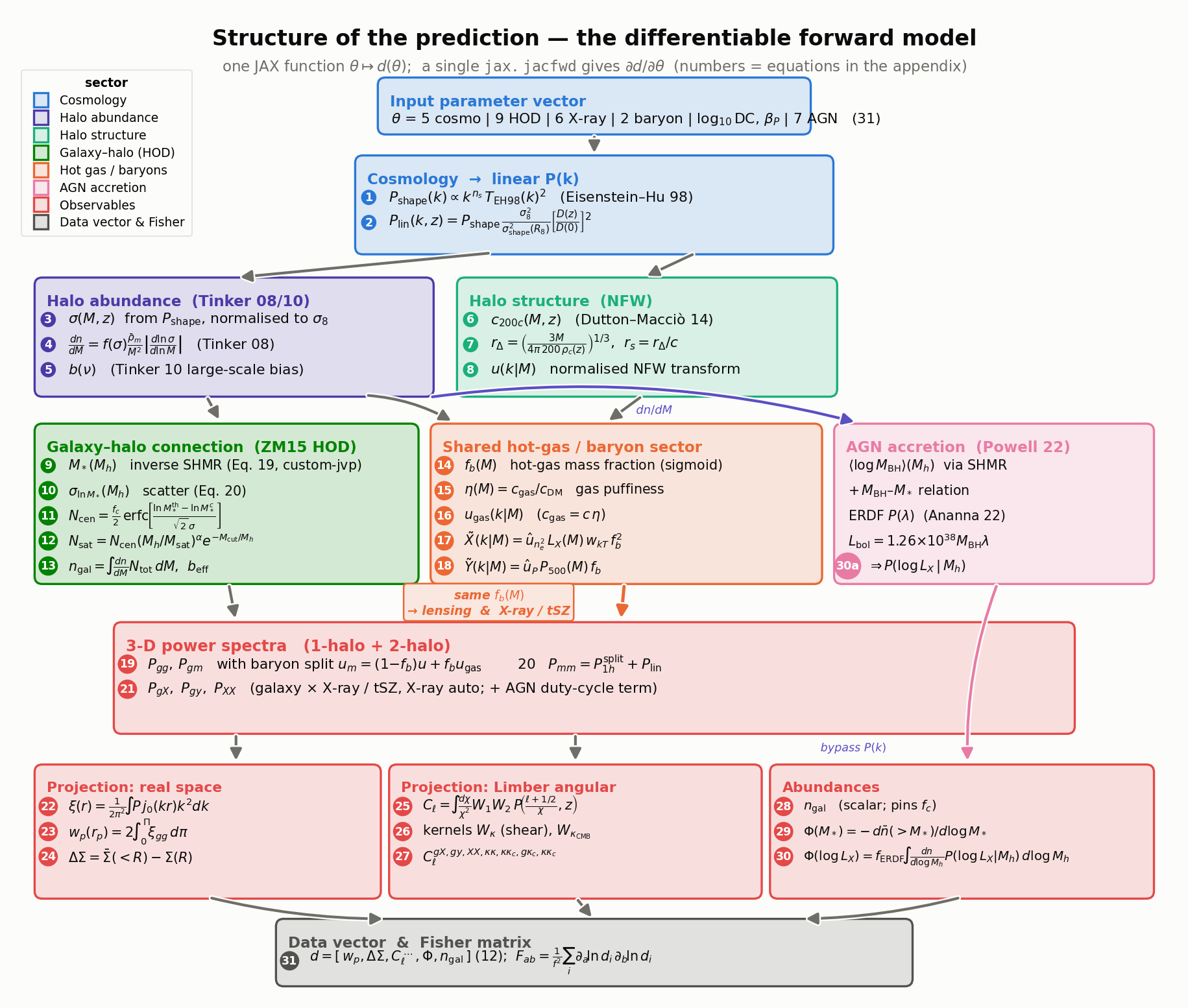
The forward model as a directed graph of equations, in evaluation order. The linear power spectrum (blue) seeds the halo abundance (violet) and halo structure (aqua); these combine with the galaxy–halo connection (green), the shared hot-gas/baryon sector (orange — the same \(f_b(M)\) drives the lensing baryon split and the X-ray/tSZ amplitudes) and the AGN accretion sector (pink) into the 3-D power spectra (red); a real-space, Limber and abundance projection then produces the twelve observables that enter the Fisher matrix. A single jax.jacfwd differentiates this entire graph at once.

A. Cosmology → linear power spectrum (pk_eisenstein_hu; inputs \(\Omega_m,\sigma_8,h,n_s,\Omega_b\)).

(1) The analytic Eisenstein & Hu (1998) transfer function gives the shape spectrum (normalised to \(P(0.05\,h/{\rm Mpc})=1\)), the one ingredient that makes the whole model JAX-traceable:

\[P_{\rm shape}(k)\propto k^{n_s}\,T_{\rm EH98}(k)^2, \qquad T_{\rm EH98}=f_b\,T_b(k)+f_c\,T_c(k).\]

(2) It is normalised to \(\sigma_8\) and evolved with the Carroll+1992 growth factor \(D(z)\) to the physical linear power used by the 2-halo term,

\[P_{\rm lin}(k,z)=P_{\rm shape}(k)\; \frac{\sigma_8^2}{\sigma^2_{\rm shape}(R_8)}\; \left[\frac{D(z)}{D(0)}\right]^2, \qquad \sigma^2(R)=\frac{1}{2\pi^2}\!\int\! P(k)\,W^2(kR)\,k^2\,dk,\]

with the real-space top-hat \(W(x)=3(\sin x-x\cos x)/x^3\).

B. Halo abundance (HaloMassFunction, Tinker08, \(\Delta=200\)).

(3) The mass variance on the shape spectrum, renormalised to \(\sigma_8\): \(\sigma(M,z)\) with \(R(M)=\big(3M/4\pi\bar\rho_m\big)^{1/3}\).

(4) The halo mass function,

\[\frac{dn}{dM}=f(\sigma)\,\frac{\bar\rho_m}{M^2}\, \left|\frac{d\ln\sigma}{d\ln M}\right|, \qquad f(\sigma)=A\!\left[\Big(\tfrac{\sigma}{b}\Big)^{-a}+1\right]e^{-c/\sigma^2} \ \text{(Tinker 08)}.\]

(5) The large-scale halo bias \(b(\nu)\), \(\nu=\delta_c/\sigma(M)\) (Tinker 10).

C. Halo structure (NFW; nfw_uk_jax()).

(6) The concentration–mass relation (Dutton & Macciò 2014),

\[\log_{10}c_{200c}=a(z)+b(z)\,\log_{10}\!\big(M/10^{12}h^{-1}M_\odot\big), \quad a=0.520+0.385\,e^{-0.617z^{1.21}},\ b=-0.101+0.026z.\]

(7) The halo radius and scale radius (comoving \(h\)-units),

\[r_\Delta=\left(\frac{3M}{4\pi\cdot 200\,\rho_c(z)}\right)^{1/3},\qquad r_s=r_\Delta/c,\qquad \rho_c(z)=\rho_{c,0}\,E^2(z)/(1+z)^3 .\]

(8) The normalised analytic NFW Fourier transform \(u(k|M)\) (→ 1 as \(k\to0\)),

\[u(k|M)=\frac{\sin(kr_s)\big[{\rm Si}((1{+}c)kr_s)-{\rm Si}(kr_s)\big] -\dfrac{\sin(ckr_s)}{(1{+}c)kr_s} +\cos(kr_s)\big[{\rm Ci}((1{+}c)kr_s)-{\rm Ci}(kr_s)\big]} {\ln(1{+}c)-c/(1{+}c)} .\]

D. Galaxy–halo connection (Zu & Mandelbaum 2015 HOD; zumandelbaum15).

(9) The inverse stellar-to-halo mass relation \(M_*(M_h)\) — the production ZM15 Eq. 19 inverted by bisection, with a custom_jvp so the gradient comes analytically from the smooth forward relation:

\[\log_{10}M_h=\log_{10}M_1+\beta\log_{10}\!\Big(\tfrac{M_*}{M_{*0}}\Big) +\frac{(M_*/M_{*0})^\delta}{1+(M_*/M_{*0})^{-\gamma}}\cdot\frac{1}{\ln 10} -\frac{1}{2\ln 10}.\]

(10) The mass-dependent scatter (Eq. 20), \(\sigma_{\ln M_*}(M_h)=\sigma_{\ln M_*,0}+\eta\,\max\!\big(0,\log_{10}(M_h/M_1)\big)\).

(11) The mean central occupation above the sample threshold (Eq. 21),

\[\langle N_{\rm cen}\rangle(M_h)=\frac{f_c}{2}\, {\rm erfc}\!\left[\frac{\big(\log_{10}M_*^{\rm thr}-\log_{10}M_*^c(M_h)\big)\ln 10} {\sqrt{2}\,\sigma_{\ln M_*}(M_h)}\right].\]

(12) The mean satellite occupation (Eq. 22),

\[\langle N_{\rm sat}\rangle(M_h)=\langle N_{\rm cen}\rangle \left(\frac{M_h}{M_{\rm sat}}\right)^{\alpha_{\rm sat}} e^{-M_{\rm cut}/M_h}, \quad M_{\rm sat}=b_{\rm sat}M_{\rm min}^{\beta_{\rm sat}},\ \ M_{\rm cut}=b_{\rm cut}M_{\rm min}^{\beta_{\rm cut}},\]

with \(M_{\rm min}(M_*^{\rm thr})\) from the forward SHMR.

(13) The occupation-weighted number density and effective bias,

\[\bar n_{\rm gal}=\!\int\! dM\,\frac{dn}{dM}\,\langle N_{\rm tot}\rangle, \qquad b_{\rm eff}=\frac{1}{\bar n_{\rm gal}}\!\int\! dM\,\frac{dn}{dM}\, \langle N_{\rm tot}\rangle\,b(M), \qquad N_{\rm tot}=N_{\rm cen}+N_{\rm sat}.\]

E. Shared hot-gas / baryon sector (BaryonFractionSigmoid).

(14) The hot-gas mass fraction — a feedback sigmoid that expels gas below the pivot \(M_{\rm pivot}\),

\[f_b(M)=f_{b,\min}+\big(\Omega_b/\Omega_m-f_{b,\min}\big)\, \frac{1}{1+\big(M_{\rm pivot}/M\big)^{\beta_b}} .\]

(15) The gas puffiness (concentration ratio \(c_{\rm gas}/c_{\rm DM}\)), \(\eta(M)=1-(1-\eta_{\min})\big/\big[1+(M/M_\eta)^{\beta_\eta}\big]\).

(16) The reduced-concentration gas NFW transform used by the ΔΣ / \(P_{mm}\) baryon split, \(u_{\rm gas}(k|M)=u_{\rm NFW}(k|M;\,c_{\rm gas}=c\,\eta)\).

F. Gas emission & pressure profiles. A spherical profile \(f(r)\) truncated at \(r_{\max}\) is Fourier-transformed by the normalised Gauss–Legendre kernel

\[\hat u(k|M)=\frac{\int_0^{r_{\max}} f(r)\,j_0(kr)\,r^2\,dr} {\int_0^{r_{\max}} f(r)\,r^2\,dr}, \qquad f_{\rm gNFW}(x)=x^{-\alpha_{\rm in}}\big(1+x^{\alpha_{\rm tr}}\big)^{(\alpha_{\rm in}-\alpha_{\rm out})/\alpha_{\rm tr}}.\]

(17) The X-ray emissivity transform: the \(n_e^2\propto f_{\rm gNFW}^2\) shape (outer slope \(\alpha_{\rm out}=\alpha_{\rm in}+2p_2\), scale \(r_s/\eta\)) times an analytic \(L_X(M)\), a weak band weight and the shared \(f_b^2\),

\[\tilde X(k|M)=\hat u_{n_e^2}(k|M)\,L_X(M)\,w_{kT}\,f_b(M)^2, \quad L_X\propto 10^{\,L_X^{\rm slope}(\log M_{500}-15)}E^2(z),\ \ w_{kT}=(kT)^{1/4}.\]

(18) The tSZ pressure transform: the Arnaud+2010 GNFW pressure shape times \(P_{500}(M)\) and the shared \(f_b\),

\[\tilde Y(k|M)=\hat u_{P}(k|M)\,P_{500}(M)\,f_b(M), \quad P_{500}\propto 10^{\,\beta_P'(\log M_{500}-14.5)}E^{8/3}(z), \ \ \beta_P'=\tfrac23+0.12+\beta_P.\]

G. Three-dimensional power spectra (halo model, 1-halo + 2-halo).

(19) Galaxy auto and galaxy–matter, the latter carrying the baryon split \(u_m=(1-f_b)\,u+f_b\,u_{\rm gas}\) (More+2015 Eqs. 9, 13):

\[P_{gg}=\frac{1}{\bar n_{\rm gal}^2}\!\int\! dM\,\frac{dn}{dM} \big(N_s^2u^2+2N_cN_su\big)+b_{\rm eff}^2P_{\rm lin},\]

\[P_{gm}=\frac{1}{\bar n_{\rm gal}}\!\int\! dM\,\frac{dn}{dM} \big(N_c+N_su\big)\frac{M}{\bar\rho_m}\,u_m+b_{\rm eff}P_{\rm lin}.\]

(20) The matter power (the cosmic-shear systematic), same baryon split:

\[P_{mm}=\int\! dM\,\frac{dn}{dM}\Big(\frac{M}{\bar\rho_m}\Big)^2 u_m^2 +P_{\rm lin}.\]

(21) The X-ray / tSZ cross and auto spectra (schematically, with \(W\in\{\tilde X,\tilde Y\}\) and a duty-cycle AGN term added to \(\tilde X\)):

\[P_{gW}=\frac{1}{\bar n_{\rm gal}}\!\int\! dM\,\frac{dn}{dM}(N_c+N_su)\,W +b_{\rm eff}P_{\rm lin}\!\int\! dM\,\frac{dn}{dM}\,b\,W,\]

\[P_{XX}=\int\! dM\,\frac{dn}{dM}\,\tilde X_{\rm tot}^2 +P_{\rm lin}\Big[\int\! dM\,\frac{dn}{dM}\,b\,\tilde X_{\rm tot}\Big]^2 .\]

H. Projection to observables.

(22) The isotropic Hankel (Ogata \(j_0\)) transform to the correlation function, \(\xi(r)=\dfrac{1}{2\pi^2}\!\int\! P(k)\,j_0(kr)\,k^2\,dk\).

(23) Projected clustering, \(w_p(r_p)=2\!\int_0^{\Pi_{\max}}\!\xi_{gg}\!\big(\sqrt{r_p^2+\pi^2}\big)\,d\pi\).

(24) Excess surface density, \(\Delta\Sigma(R)=\bar\Sigma(<R)-\Sigma(R)\), with \(\Sigma(R)=\bar\rho_m\!\int\!\xi_{gm}\!\big(\sqrt{R^2+\chi^2}\big)\,d\chi\) and \(\bar\Sigma(<R)=\tfrac{2}{R^2}\!\int_0^R\!R'\,\Sigma(R')\,dR'\).

(25) The angular spectra via the Limber approximation,

\[C_\ell=\int\! d\chi\,\frac{W_1(\chi)\,W_2(\chi)}{\chi^2}\, P\!\left(k=\frac{\ell+1/2}{\chi},\,z(\chi)\right).\]

(26) The projection kernels: the galaxy window \(W_g=dN/d\chi\) (narrow \(n(z)\) shell), the cosmic-shear efficiency and the CMB-lensing kernel (single source plane at \(z_*\simeq1089\)),

\[W_\kappa(\chi)=\tfrac32\Omega_m\Big(\tfrac{H_0}{c}\Big)^2\frac{\chi}{a} \!\int_\chi^{\chi_H}\!\! d\chi'\,n_s(\chi')\frac{\chi'-\chi}{\chi'}, \qquad W_{\kappa_{\rm CMB}}(\chi)=\tfrac32\Omega_m\Big(\tfrac{H_0}{c}\Big)^2 \frac{\chi}{a}\,\frac{\chi_*-\chi}{\chi_*}.\]

(27) The seven realised angular spectra: \(C_\ell^{gX},C_\ell^{gy}, C_\ell^{XX}\) (galaxy-window × gas), \(C_\ell^{\kappa\kappa}\) (cosmic-shear auto), \(C_\ell^{\kappa_c\kappa_c}\) (CMB-lensing auto), \(C_\ell^{g\kappa_c}\) (galaxy × CMB-lensing) and \(C_\ell^{\kappa\kappa_c}\) (shear × CMB-lensing).

I. Abundance observables.

(28) The galaxy number density (a scalar; the observable that pins \(f_c\)), \(\bar n_{\rm gal}=\int\! dM\,\frac{dn}{dM}\,\langle N_{\rm tot}\rangle\).

(29) The stellar-mass function, \(\Phi(M_*)=-\,d\bar n(>\!M_*)/d\log_{10}M_*\).

(30) The AGN X-ray luminosity function (Powell 2022): the ZM15 SHMR → a free \(M_{\rm BH}\)–\(M_*\) relation → a universal Eddington-ratio distribution (Ananna 2022) build the per-halo kernel \(P(\log L_X|M_h)\) (a shift-invariant ERDF ⊛ Gaussian), integrated over the mass function:

\[\Phi(\log L_X)=f_{\rm ERDF}\!\int\! d\log M_h\; \frac{dn}{d\log M_h}(\Omega_m,\sigma_8)\;P(\log L_X\,|\,M_h).\]

J. Data vector and Fisher matrix.

(31) The twelve observables are concatenated into the data vector \(d(\theta)=\big[\,w_p,\Delta\Sigma,C_\ell^{gX},C_\ell^{gy},C_\ell^{XX}, C_\ell^{\kappa\kappa},C_\ell^{\kappa_c\kappa_c},C_\ell^{g\kappa_c}, C_\ell^{\kappa\kappa_c},\Phi(L_X),\bar n_{\rm gal},\Phi(M_*)\,\big]\), and — with a constant relative error \(f\) — the Fisher matrix is the single jax.jacfwd Jacobian contracted against the diagonal covariance,

\[F_{ab}=\sum_i\frac{1}{(f\,d_i)^2} \frac{\partial d_i}{\partial\theta_a}\frac{\partial d_i}{\partial\theta_b} =\frac{1}{f^2}\sum_i \frac{\partial\ln d_i}{\partial\theta_a}\frac{\partial\ln d_i}{\partial\theta_b},\]

closing the loop with the Fisher identity used at the top of this page (an analytic Gaussian covariance with cross-observable correlations is available via hod_mod.forecast.covariance).