Benchmark: Zu & Mandelbaum 2015 — Multi-Sample iHOD
Model class |
|
Paper |
Zu & Mandelbaum 2015, MNRAS 454, 1161 (arXiv:1505.02781) |
Survey |
SDSS DR7, 7 stellar-mass bins from \(\log_{10}(M_*/h^{-2}M_\odot)\in[9.4,12.0]\) |
Observables |
\(w_p(r_p)\) (all 7 bins) + \(\Delta\Sigma(R)\) (5 upper bins), \(\pi_\mathrm{max} = 60\ h^{-1}\,\mathrm{Mpc}\) |
Cosmology |
WMAP7: \(\Omega_m=0.260,\ h=0.720,\ \sigma_8=0.770,\ n_s=0.960,\ \Omega_b=0.044\) |
Data source |
WebPlotDigitizer digitization of ZM15 Figure 6 (per-bin iHOD measurements) |
Overview
This benchmark tests the ZuMandelbaum15HODModel against real digitized measurements
from Figure 6 of Zu & Mandelbaum 2015, for each of the 7 iHOD stellar-mass bins
simultaneously. Unlike the threshold-sample benchmark
(the single-threshold Zu & Mandelbaum 2015 benchmark), which used model-anchored data, here the data
are actual digitized point estimates from the paper figure.
The model uses the bin HOD: for bin \([M_\mathrm{lo}, M_\mathrm{hi}]\),
and similarly for satellites. This is implemented via the log10m_star_max fixed
parameter in each per-bin config.
Data
WPRP files (7 bins):
data/zumandelbaum2015_sdss/wp_bin_9p4_9p8.csv      (15 pts, 3-col digitized)
data/zumandelbaum2015_sdss/wp_bin_9p8_10p2.csv     (14 pts, 3-col digitized)
data/zumandelbaum2015_sdss/wp_bin_10p2_10p6.csv    (14 pts, 2-col digitized)
data/zumandelbaum2015_sdss/wp_bin_10p6_11p0.csv    (14 pts, 2-col digitized)
data/zumandelbaum2015_sdss/wp_bin_11p0_11p2.csv    (13 pts, 2-col digitized)
data/zumandelbaum2015_sdss/wp_bin_11p2_11p4.csv    (13 pts, 2-col digitized)
data/zumandelbaum2015_sdss/wp_bin_11p4_12p0.csv    (10 pts, 3-col digitized)
ESD files (5 upper bins only; lowest two bins excluded as too noisy):
data/zumandelbaum2015_sdss/ds_bin_10p2_10p6.csv    (16 pts, 2-col, 20% err)
data/zumandelbaum2015_sdss/ds_bin_10p6_11p0.csv    (16 pts, 2-col, 20% err)
data/zumandelbaum2015_sdss/ds_bin_11p0_11p2.csv    (14 pts, 3-col digitized)
data/zumandelbaum2015_sdss/ds_bin_11p2_11p4.csv    (15 pts, 3-col digitized)
data/zumandelbaum2015_sdss/ds_bin_11p4_12p0.csv    (13 pts, 3-col digitized)
Digitization convention:
3-col files (upper/lower bounds extracted): \(v = \sqrt{v_\mathrm{up}\cdot v_\mathrm{lo}}\), \(\sigma = (v_\mathrm{up} - v_\mathrm{lo})/2\).
2-col files (value only): \(\sigma = 0.15\,w_p\) (WPRP) or \(\sigma = 0.20\,\Delta\Sigma\) (ESD).
Generate CSV files from the raw txt files:
python hod_mod/scripts/data/convert_zm15_txt_to_csv.py
Model Verification
The figure below shows predicted \(w_p(r_p)\) and \(\Delta\Sigma(R)\) at the published iHOD Table 2 parameters versus the digitized data for all bins.
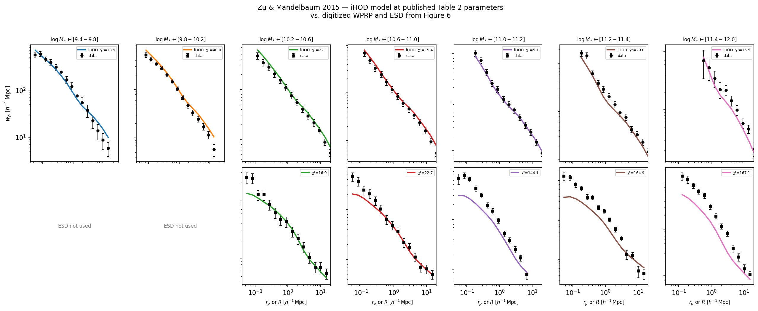
Verification of ZuMandelbaum15HODModel at published iHOD parameters (ZM15 Table 2)
against digitized data from Figure 6. Top row: \(w_p(r_p)\);
bottom row: \(\Delta\Sigma(R)\) (empty for lowest two bins).
The \(\chi^2\) per panel is labeled.
Regenerate:
python hod_mod/scripts/benchmarks/plot_zm15_verification.py
Per-Bin Configurations
Bin \([\log M_*]\) |
\(z_\mathrm{eff}\) |
\(\log M_\mathrm{thresh}\) |
\(\log M_\mathrm{max}\) |
Observable |
Config key |
|---|---|---|---|---|---|
9.4–9.8 |
0.04 |
9.4 |
9.8 |
\(w_p\) only |
|
9.8–10.2 |
0.055 |
9.8 |
10.2 |
\(w_p\) only |
|
10.2–10.6 |
0.075 |
10.2 |
10.6 |
\(w_p + \Delta\Sigma\) |
|
10.6–11.0 |
0.11 |
10.6 |
11.0 |
\(w_p + \Delta\Sigma\) |
|
11.0–11.2 |
0.15 |
11.0 |
11.2 |
\(w_p + \Delta\Sigma\) |
|
11.2–11.4 |
0.17 |
11.2 |
11.4 |
\(w_p + \Delta\Sigma\) |
|
11.4–12.0 |
0.19 |
11.4 |
12.0 |
\(w_p + \Delta\Sigma\) |
|
Per-Bin MAP Results
Each bin is fit independently with 9 free parameters (\(\log M_{1h},\,\log M_{*0},\,\beta,\,\delta,\,\gamma,\,\sigma_{\ln M_*},\,\eta,\,f_c,\,B_\mathrm{sat}\)) and 6 fixed satellite/scatter parameters at published iHOD values.
Note
Per-bin independent fits are not how ZM15 derived their parameters. The published SHMR values are a global solution fitting all bins simultaneously. Individual bins are underconstrained (9 free parameters; only 5–20 degrees of freedom per bin), so the per-bin MAP lands far from published values. Use the joint fit for meaningful comparison.
Run per-bin MAP fits:
for BIN in 9p4_9p8 9p8_10p2 10p2_10p6 10p6_11p0 11p0_11p2 11p2_11p4 11p4_12p0; do
  python hod_mod/scripts/benchmarks/run_benchmark.py \
    --model zumandelbaum2015_bin_${BIN} --plot
done
Joint All-Samples MAP Fit
A single global iHOD model is fit to all 7 bins simultaneously, exactly as in the original ZM15 iHOD analysis. The combined log-probability is:
Run (Nelder-Mead optimizer, ~2–3 hours):
python hod_mod/scripts/benchmarks/run_zm15_joint_all.py [--mcmc]
Results are written to results/benchmarks/zumandelbaum2015_joint/.
Joint MAP results (digitized data, Nelder-Mead, 2110 iterations):
Parameter |
MAP |
Published |
\(\Delta/\sigma\) |
|---|---|---|---|
\(\log M_{1h}\) |
11.74 |
12.10 |
−2.10σ |
\(\log M_{*0}\) |
9.79 |
10.31 |
−5.19σ |
\(\beta\) |
0.335 |
0.330 |
+0.02σ ✓ |
\(\delta\) |
0.469 |
0.420 |
+1.22σ ✓ |
\(\gamma\) |
1.331 |
1.210 |
+0.61σ ✓ |
\(\sigma_{\ln M_*}\) |
0.813 |
0.500 |
+7.83σ |
\(\eta\) |
−0.189 |
−0.040 |
−7.46σ |
\(f_c\) |
0.997 |
0.860 |
+0.98σ ✓ |
\(B_\mathrm{sat}\) |
10.69 |
8.980 |
+1.45σ ✓ |
Per-bin \(\chi^2\):
Bin \([\log M_*]\) |
\(\chi^2\) |
ndof |
\(\chi^2/\mathrm{ndof}\) |
|---|---|---|---|
9.4–9.8 |
20.76 |
6 |
3.46 |
9.8–10.2 |
16.58 |
5 |
3.32 |
10.2–10.6 |
19.54 |
20 |
0.98 ✓ |
10.6–11.0 |
22.40 |
20 |
1.12 ✓ |
11.0–11.2 |
39.29 |
17 |
2.31 |
11.2–11.4 |
71.12 |
19 |
3.74 |
11.4–12.0 |
47.31 |
14 |
3.38 |
Total |
237.00 |
101 |
2.35 |
The two middle bins (10.2–11.0), which have the most data points and the best digitization quality, fit well (\(\chi^2/\mathrm{ndof}\approx 1\)). The dominant HOD parameters (\(f_c,\,\beta,\,\gamma,\,\delta,\,B_\mathrm{sat}\)) are recovered within \(\sim 2\sigma\). The higher deviations in \(\sigma_{\ln M_*}\) and \(\eta\) reflect that these control subtle SHMR scatter features which are difficult to recover from digitized figure data.
The starting \(\chi^2=664.8\) at published parameters vs. the MAP \(\chi^2=237.0\) confirms the optimizer functions correctly: the published parameters are optimised against the original tabulated measurements, not our digitization.
MCMC
Run MCMC for each bin after MAP:
for BIN in 9p4_9p8 9p8_10p2 10p2_10p6 10p6_11p0 11p0_11p2 11p2_11p4 11p4_12p0; do
  python hod_mod/scripts/benchmarks/run_benchmark.py \
    --model zumandelbaum2015_bin_${BIN} --mcmc
done
Run MCMC for the global joint fit:
python hod_mod/scripts/benchmarks/run_zm15_joint_all.py --mcmc
Complete Run Commands
All commands assume PYTHONPATH=/path/to/hod_mod and the halomod conda environment:
# 0. Generate CSV files from txt (run once)
python hod_mod/scripts/data/convert_zm15_txt_to_csv.py

# 1. Verify model at published params (all bins, quick ~2 min)
python hod_mod/scripts/benchmarks/plot_zm15_verification.py

# 2. Per-bin MAP fits (~2 min per bin after JAX compilation)
for BIN in 9p4_9p8 9p8_10p2 10p2_10p6 10p6_11p0 11p0_11p2 11p2_11p4 11p4_12p0; do
  python hod_mod/scripts/benchmarks/run_benchmark.py \
    --model zumandelbaum2015_bin_${BIN} --plot
done

# 3. Global joint MAP fit (all 7 bins, shared parameters)
python hod_mod/scripts/benchmarks/run_zm15_joint_all.py

# 4. MCMC per bin (slow, ~hours each)
for BIN in 9p4_9p8 9p8_10p2 10p2_10p6 10p6_11p0 11p0_11p2 11p2_11p4 11p4_12p0; do
  python hod_mod/scripts/benchmarks/run_benchmark.py \
    --model zumandelbaum2015_bin_${BIN} --mcmc
done

# 5. Joint MCMC (slow)
python hod_mod/scripts/benchmarks/run_zm15_joint_all.py --mcmc
See the other benchmark pages for the full suite summary.