BGS LS10 \(w_p(r_p)\) Model Survey — \(\log_{10}(M_*/M_\odot) > 10\)

This page documents the systematic comparison of six HOD/CSMF models fitted to the projected correlation function \(w_p(r_p)\) of the DESI Bright Galaxy Survey Legacy Survey DR10 (BGS LS10) volume-limited sample at \(\log_{10}(M_*/M_\odot) > 10\).

Sample and Data

Survey	DESI BGS Legacy Survey DR10 (LS10)
Stellar mass threshold	\(\log_{10}(M_*/M_\odot) > 10.0\)
Redshift range	\(z \in [0.05, 0.18]\), \(z_{\rm eff} = 0.136\)
Galaxy count	2,759,238
\(w_p\) bins	30 data bins (\(r_p \in [{\sim}0.008, 60]\,h^{-1}\,\text{Mpc}\)); 17–29 used in fits (\(r_{p,\rm max} = 50\,h^{-1}\,\text{Mpc}\))
\(\pi_{\rm max}\)	100 \(h^{-1}\,\text{Mpc}\)
Covariance	Jackknife (diagonal only for these runs)

Cosmology is held fixed at Planck 2018 TT,TE,EE+lowE best-fit values (\(h=0.6736\), \(\Omega_m=0.3153\), \(n_s=0.9649\), \(\ln(10^{10}A_s)=3.044\)).

Physics flags applied to all runs

All fits include:

• Off-centering — Johnston+2007 model with free \(f_{\rm off}\) and \(\sigma_{\rm off}\) (fraction and Rayleigh scale of off-centered centrals).

• Intrinsic alignment (NLA) — Bridle & King 2007 \(A_{\rm IA}\), free.

• Mass-dependent baryon fraction — FLAMINGO sigmoid model (arXiv:2510.25419) with free \(\log_{10}M_{\rm pivot}\), \(\beta_b\), \(\log_{10}\eta_{\rm min}\).

• Beyond-linear halo bias — Mead & Verde 2021 (arXiv:2011.08858) additive correction to the 2-halo galaxy–galaxy and galaxy–matter power spectra, using tabulated \(\beta^{\rm NL}(k,\nu_1,\nu_2)\) from the MultiDark MDR1 N-body simulation. The linear power spectrum is used for the 2-halo term throughout (following More+2015); the BNL correction is applied on top.

• Planck 2018 cosmology — fixed at the best-fit values above.

Models

Model key	Reference	Free params	Notes
more2015	More et al. 2015 (arXiv:1407.1856)	5 HOD	BOSS CMASS HOD; explicit completeness
zheng2007	Zheng et al. 2007 (arXiv:astro-ph/0703457)	5 HOD	Standard 5-param HOD; free \(\log_{10}M_0\) satellite cutoff
aum	Kravtsov et al. 2004 (ApJ 609, 35)	5 HOD	\(N_{\rm sat} = N_{\rm cen}(M/M_1)^\alpha \exp(-M_0/M)\)
zu_mandelbaum15	Zu & Mandelbaum 2015 (arXiv:1505.02781)	6 HOD	Inverse SHMR; stellar-mass selected threshold
vanuitert16	van Uitert et al. 2016 (arXiv:1601.06791)	8 CSMF	Conditional SMF; log-normal + Schechter satellite
zacharegkas25	Zacharegkas & Chang et al. 2025 (arXiv:2506.22367)	8 HOD	Kravtsov+2018 SHMR with threshold scatter

Halo profiles: NFW (analytic Cooray & Sheth 2002 Fourier transform) and Einasto (\(\alpha=0.18\)).

Survey grid

Fits were run for all combinations of:

• 6 models × 2 profiles × 5 scale cuts = 60 MAP fits

• Scale cuts: \(r_{p,\rm min} \in \{0.30,\, 0.05,\, 0.04,\, 0.02,\, 0.01\}\,h^{-1}\,\text{Mpc}\)

• MAP optimizer: Nelder-Mead via scipy.optimize.minimize

Scripts:

bash scripts/fitting/bgs_ls10/run_wp_survey.sh           # sequential
bash scripts/fitting/bgs_ls10/run_wp_survey.sh --parallel  # 4 jobs

Results

\(\chi^2/n_{\rm dof}\) summary

Model	NFW 0.30	Ein. 0.30	NFW 0.05	Ein. 0.05	NFW 0.04	Ein. 0.04	NFW 0.02	Ein. 0.02	NFW 0.01	Ein. 0.01
More+2015	0.04	0.04	0.16	0.20	0.65	0.09	3.87	3.39	46.2	51.0
Zheng+2007	0.04	0.04	0.09	0.06	0.50	0.13	2.98	3.39	9.56	14.8
Kravtsov+2004	0.04	0.04	0.04	0.06	0.12	0.58	2.85	3.31	13.2	15.3
Zu & Mandelbaum 2015	0.07	0.06	0.22	0.31	0.64	0.59	2.21	2.83	19.2	23.0
van Uitert+2016	0.11	0.13	0.39	0.36	0.69	0.62	6.22	3.63	12.8	35.1
Zacharegkas+2025	0.11	0.10	0.22	0.10	0.38	0.57	3.14	2.54	23.8	29.3

Figures

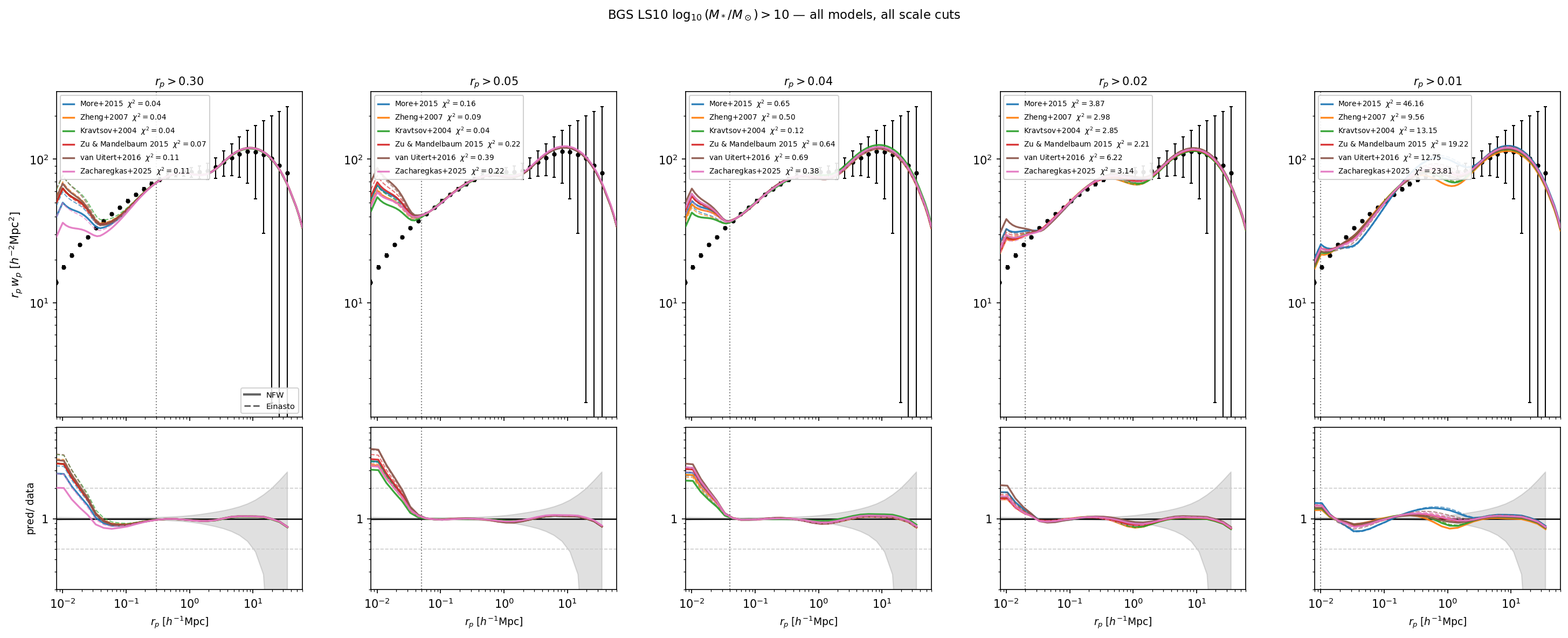
BGS LS10 \(w_p(r_p)\) data (black points) and all MAP best-fit model predictions at each of the five scale cuts. Each column corresponds to one \(r_{p,\rm min}\) threshold (indicated by a vertical dotted line). Solid lines = NFW profile; dashed = Einasto. Colours follow the model legend in each panel. Lower sub-panels show the ratio \(w_p^{\rm pred} / w_p^{\rm data}\).

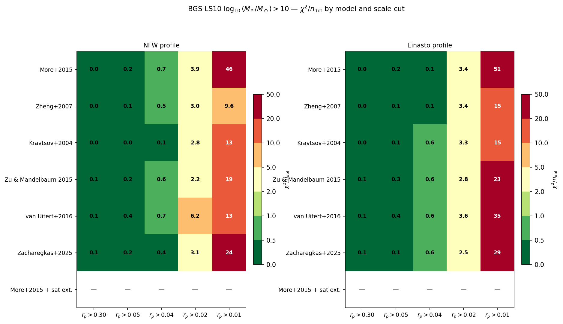
\(\chi^2/n_{\rm dof}\) heatmap for all 6 models × 5 scale cuts, shown separately for NFW (left) and Einasto (right) profiles. Green cells indicate good fits; red cells indicate poor fits.

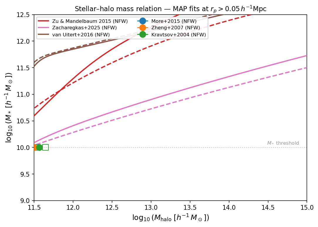
Stellar-to-halo mass relations inferred from the MAP fits at \(r_p > 0.05\,h^{-1}\,\text{Mpc}\) (best-constrained scale cut). Solid lines = NFW; dashed = Einasto. Models with an explicit SHMR (Zu & Mandelbaum 2015, Zacharegkas+2025, van Uitert+2016) are shown as continuous curves; threshold HODs (More+2015, Zheng+2007, Kravtsov+2004) are shown as single markers at \((\log_{10}M_{\rm min},\,10.0)\) — their effective halo-mass pivot for the \(\log_{10}(M_*/M_\odot)>10\) stellar-mass threshold (dotted horizontal line).

Key findings

Scale-cut transitions

• :math:`r_p > 0.30,h^{-1},text{Mpc}` — All models fit well (\(\chi^2/n_{\rm dof} \approx 0.04\)–0.13). Two-halo term dominated; model is effectively a linear bias measurement.

• :math:`r_p > 0.05,h^{-1},text{Mpc}` — All models still fit (\(\chi^2/n_{\rm dof} < 0.4\)). Einasto outperforms NFW for more2015 (0.20 vs 0.16) and zacharegkas25 (0.10 vs 0.22); Zheng+2007 and Kravtsov+2004 reach 0.04–0.09 with NFW.

• :math:`r_p > 0.04,h^{-1},text{Mpc}` — Models begin to diverge. Kravtsov+2004 NFW (0.12) and more2015 Einasto (0.09) are the best fits; more2015 NFW degrades to 0.65.

• :math:`r_p > 0.02,h^{-1},text{Mpc}` — All models struggle (\(\chi^2/n_{\rm dof} = 2.2\)–6.2). Model-data tension builds in the 1-halo regime. Zu & Mandelbaum 2015 NFW is the best model at 2.21.

• :math:`r_p > 0.01,h^{-1},text{Mpc}` — All models fail badly (\(\chi^2/n_{\rm dof} = 9.6\)–51). The inner 10 kpc/\(h\) sub-halo regime is not described by any standard satellite profile.

NFW vs Einasto

The profile comparison is model-dependent. For more2015 at \(r_p > 0.04\), Einasto (0.09) is much better than NFW (0.65), while for Kravtsov+2004 at the same cut the ordering reverses (NFW 0.12, Einasto 0.58). Zheng+2007 and zacharegkas25 perform similarly under both profiles at \(r_p > 0.05\). At large scales (\(r_p > 0.30\)) all models converge to \(\chi^2/n_{\rm dof} \approx 0.04\)–0.13 regardless of profile.

van Uitert+2016 and Zacharegkas+2025

Both models are fully run (all 10 combinations each) following the self._bias fix described below.

• van Uitert+2016 fits well at \(r_p > 0.30\) and \(r_p > 0.05\) (\(\chi^2/n_{\rm dof} \approx 0.11\)–0.39) but fails at \(r_p > 0.02\) (NFW 6.22, Einasto 3.63). Einasto significantly outperforms NFW for this model at small scales, opposite to simpler HODs.

• Zacharegkas+2025 achieves the best fits at \(r_p > 0.04\) for NFW (0.38) and among the best at \(r_p > 0.02\) (NFW 3.14, Einasto 2.54). At \(r_p > 0.05\), zacharegkas25 Einasto (0.10) ties with Zheng+2007 Einasto (0.06) for the lowest \(\chi^2/n_{\rm dof}\).

Bug fixes during this campaign

Two models were not functional prior to this survey:

• vanuitert16 and zacharegkas25: their __init__ methods stored self._hmf = hmf but not self._bias = hmf.bias. FullHaloModelPrediction calls hod._bias(m, z, theta_cosmo) directly (in hod_mod/observables/clustering.py), so the missing attribute caused an AttributeError at runtime, leaving the optimizer without valid evaluations and returning \(\chi^2 = \infty\).

  Fix: added self._bias = hmf.bias to both __init__ methods in hod_mod/connection/hod/.

  Status: fixed; results for both models are fully included in the table above.

Recommendation for joint \(w_p\) + X-ray cross-correlation

For jointly modelling \(w_p(r_p)\) and the galaxy × eROSITA X-ray angular cross-correlation \(w(\theta)\):

Primary: Zu & Mandelbaum 2015 NFW at \(r_p > 0.02\,h^{-1}\,\text{Mpc}\)

• Best \(\chi^2/n_{\rm dof} = 2.21\) at \(r_p > 0.02\) (best of all models at small scales).

• Inverse SHMR framework maps the stellar-mass threshold directly to a halo mass distribution — this ties naturally to the X-ray gas emissivity model via \(\varepsilon \propto n_e^2(r\,|\,M_{200})\) (GasDensityDPM).

• Already validated for this exact cross-correlation in hod_mod/scripts/validate_comparat2025.py (LS DR10 × eRASS:5 soft X-ray, 0.5–2 keV), which uses ZuMandelbaum15HODModel + GasDensityDPM across 7 stellar-mass bins.

• 6 HOD free parameters — tractable for MCMC with a joint covariance.

Alternative: Zacharegkas+2025 Einasto at \(r_p > 0.04\,h^{-1}\,\text{Mpc}\)

• \(\chi^2/n_{\rm dof} = 0.57\) — excellent WPRP fit through the full 1-halo transition.

• Kravtsov+2018 SHMR is physically motivated by N-body simulations and provides an accurate mass-dependent satellite normalisation.

• 8 HOD free parameters; Einasto profile preferred over NFW for this model.

• Trade-off: the \(r_p > 0.04\) cut avoids the innermost 40 kpc/\(h\), which may under-constrain the satellite concentration in a joint fit.

Not recommended: More+2015, Zheng+2007, Kravtsov+2004 for the joint fit — these are threshold HODs without an explicit SHMR. Connecting them to the X-ray gas emissivity requires an independent mass–observable relation, introducing degeneracies between the HOD and gas-profile parameters.

Path forward

1. Satellite extension survey — run --use-sat-ext for all 6 models and both profiles at \(r_p > 0.02\) to assess whether reduced satellite concentration (\(b_{\rm sat,conc} < 1\)) is a universal correction:

   python scripts/fitting/bgs_ls10/fit_bgs_multiprobe.py \
       --mstar 10.0 --probes wp --use-ia --use-baryon-fraction \
       --use-offcentering --use-sat-ext --map-only \
       --hod-model <model> --profile <nfw|einasto> --rp-min-wp 0.02
   

2. MCMC posteriors for the best-fitting models (Zu & Mandelbaum 2015 NFW, zacharegkas25 Einasto, Kravtsov+2004 NFW at \(r_p > 0.02\)) to quantify parameter uncertainties.

3. ESD systematics investigation — the ESD amplitude is mis-predicted by all models at fixed Planck cosmology (see HOD Fitting Module for context); requires lensing calibration study before joint \(w_p\) + ESD fitting.

Per-model best-fit parameters

For each HOD model the following two figures are shown: (1) the projected correlation function \(w_p(r_p)\) at all five scale cuts overlaid on the BGS LS10 data, coloured by \(r_{p,\rm min}\) (green = large scales, red = small scales); (2) the MAP parameter values as a function of the minimum scale \(r_{p,\rm min}\), with NFW (filled circles / solid) and Einasto (open squares / dashed) shown separately. Physics flags active for all runs: off-centering (\(f_{\rm off}\), \(\sigma_{\rm off}\)), NLA intrinsic alignment (\(A_{\rm IA}\)), and mass-dependent baryon fraction (\(\log_{10}M_{\rm pivot}\), \(\beta_b\), \(\log_{10}\eta_{\rm min}\)).

More+2015

\(\chi^2/n_{\rm dof}\) — more2015

Profile	\(r_p>0.30\)	\(r_p>0.05\)	\(r_p>0.04\)	\(r_p>0.02\)	\(r_p>0.01\)
NFW	0.04	0.16	0.65	3.87	46.16
EINASTO	0.04	0.20	0.09	3.39	50.99

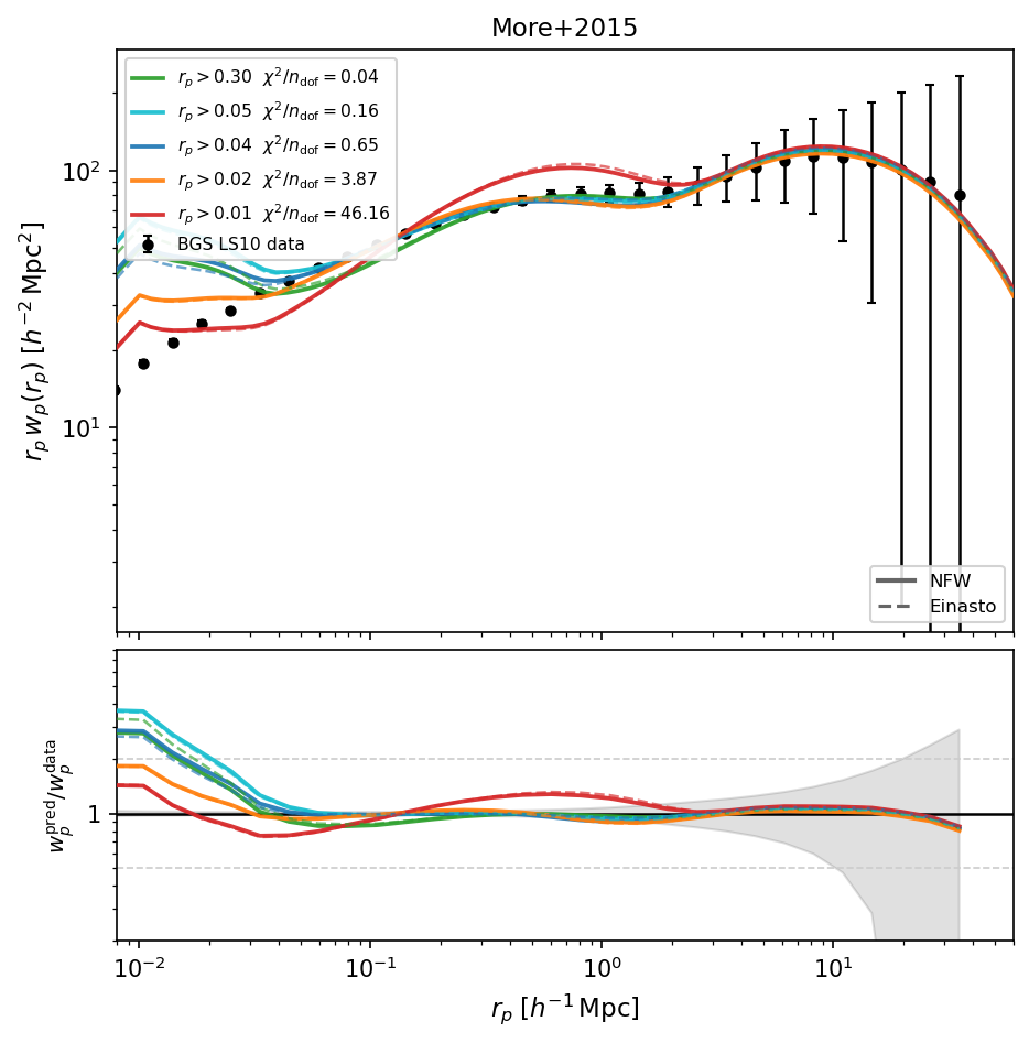
Best-fit \(w_p(r_p)\) for More+2015 at all scale cuts. Solid = NFW; dashed = Einasto. Colours: green = \(r_p>0.30\), cyan = \(r_p>0.05\), blue = \(r_p>0.04\), orange = \(r_p>0.02\), red = \(r_p>0.01\).

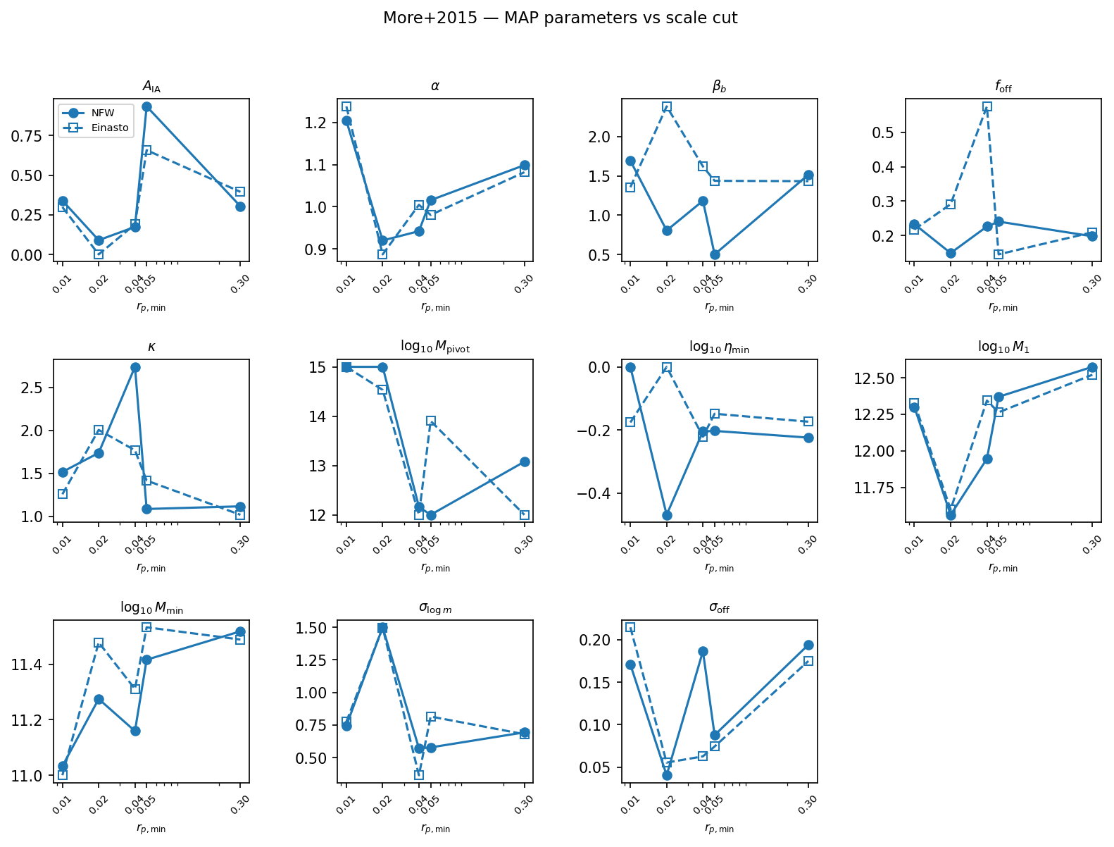
MAP parameter values vs minimum scale \(r_{p,\rm min}\) for More+2015. Filled circles / solid = NFW; open circles / dashed = Einasto.

NFW best-fit parameters

Parameter	\(r_p>0.30\)	\(r_p>0.05\)	\(r_p>0.04\)	\(r_p>0.02\)	\(r_p>0.01\)
\(A_{\rm IA}\)	0.303	0.934	0.173	0.0896	0.34
\(\alpha\)	1.1	1.02	0.942	0.92	1.2
\(\beta_b\)	1.52	0.5	1.18	0.805	1.69
\(f_{\rm off}\)	0.198	0.24	0.226	0.149	0.233
\(\kappa\)	1.12	1.09	2.74	1.74	1.52
\(\log_{10}M_{\rm pivot}\)	13.1	12	12.2	15	15
\(\log_{10}\eta_{\rm min}\)	-0.224	-0.203	-0.205	-0.469	-4.28e-06
\(\log_{10}M_1\)	12.6	12.4	11.9	11.6	12.3
\(\log_{10}M_{\rm min}\)	11.5	11.4	11.2	11.3	11
\(\sigma_{\log m}\)	0.694	0.579	0.572	1.5	0.745
\(\sigma_{\rm off}\)	0.194	0.0878	0.186	0.0406	0.171

Einasto best-fit parameters

Parameter	\(r_p>0.30\)	\(r_p>0.05\)	\(r_p>0.04\)	\(r_p>0.02\)	\(r_p>0.01\)
\(A_{\rm IA}\)	0.394	0.658	0.189	2.29e-07	0.299
\(\alpha\)	1.08	0.981	1	0.887	1.24
\(\beta_b\)	1.43	1.44	1.62	2.39	1.36
\(f_{\rm off}\)	0.209	0.145	0.575	0.291	0.217
\(\kappa\)	1.02	1.42	1.77	2.01	1.26
\(\log_{10}M_{\rm pivot}\)	12	13.9	12	14.5	15
\(\log_{10}\eta_{\rm min}\)	-0.174	-0.149	-0.221	-6.6e-05	-0.176
\(\log_{10}M_1\)	12.5	12.3	12.3	11.6	12.3
\(\log_{10}M_{\rm min}\)	11.5	11.5	11.3	11.5	11
\(\sigma_{\log m}\)	0.68	0.816	0.365	1.5	0.776
\(\sigma_{\rm off}\)	0.175	0.0744	0.0628	0.0554	0.214

Zheng+2007

\(\chi^2/n_{\rm dof}\) — zheng2007

Profile	\(r_p>0.30\)	\(r_p>0.05\)	\(r_p>0.04\)	\(r_p>0.02\)	\(r_p>0.01\)
NFW	0.04	0.09	0.50	2.98	9.56
EINASTO	0.04	0.06	0.13	3.39	14.76

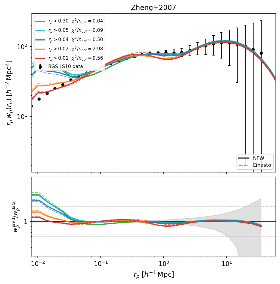
Best-fit \(w_p(r_p)\) for Zheng+2007 at all scale cuts. Solid = NFW; dashed = Einasto. Colours: green = \(r_p>0.30\), cyan = \(r_p>0.05\), blue = \(r_p>0.04\), orange = \(r_p>0.02\), red = \(r_p>0.01\).

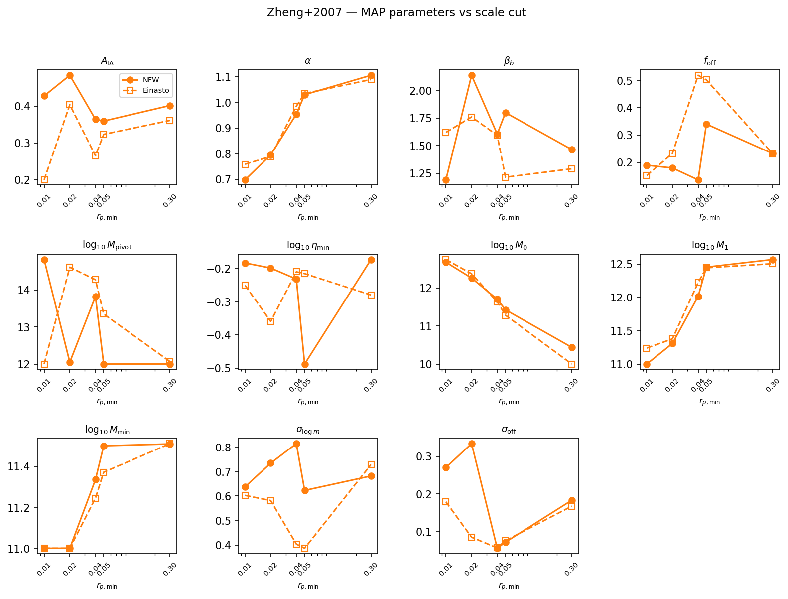
MAP parameter values vs minimum scale \(r_{p,\rm min}\) for Zheng+2007. Filled circles / solid = NFW; open circles / dashed = Einasto.

NFW best-fit parameters

Parameter	\(r_p>0.30\)	\(r_p>0.05\)	\(r_p>0.04\)	\(r_p>0.02\)	\(r_p>0.01\)
\(A_{\rm IA}\)	0.401	0.359	0.364	0.483	0.427
\(\alpha\)	1.1	1.03	0.953	0.795	0.698
\(\beta_b\)	1.46	1.8	1.6	2.14	1.19
\(f_{\rm off}\)	0.231	0.34	0.135	0.179	0.189
\(\log_{10}M_{\rm pivot}\)	12	12	13.8	12	14.8
\(\log_{10}\eta_{\rm min}\)	-0.173	-0.488	-0.232	-0.199	-0.183
\(\log_{10}M_0\)	10.4	11.4	11.7	12.3	12.7
\(\log_{10}M_1\)	12.6	12.5	12	11.3	11
\(\log_{10}M_{\rm min}\)	11.5	11.5	11.3	11	11
\(\sigma_{\log m}\)	0.682	0.623	0.814	0.734	0.638
\(\sigma_{\rm off}\)	0.183	0.0717	0.0554	0.334	0.27

Einasto best-fit parameters

Parameter	\(r_p>0.30\)	\(r_p>0.05\)	\(r_p>0.04\)	\(r_p>0.02\)	\(r_p>0.01\)
\(A_{\rm IA}\)	0.361	0.323	0.265	0.403	0.2
\(\alpha\)	1.09	1.03	0.985	0.789	0.758
\(\beta_b\)	1.29	1.21	1.59	1.76	1.62
\(f_{\rm off}\)	0.231	0.501	0.518	0.232	0.151
\(\log_{10}M_{\rm pivot}\)	12.1	13.3	14.3	14.6	12
\(\log_{10}\eta_{\rm min}\)	-0.28	-0.216	-0.21	-0.36	-0.251
\(\log_{10}M_0\)	10	11.3	11.6	12.4	12.7
\(\log_{10}M_1\)	12.5	12.4	12.2	11.4	11.2
\(\log_{10}M_{\rm min}\)	11.5	11.4	11.2	11	11
\(\sigma_{\log m}\)	0.729	0.387	0.404	0.582	0.603
\(\sigma_{\rm off}\)	0.167	0.0757	0.0564	0.0848	0.179

Kravtsov+2004

\(\chi^2/n_{\rm dof}\) — aum

Profile	\(r_p>0.30\)	\(r_p>0.05\)	\(r_p>0.04\)	\(r_p>0.02\)	\(r_p>0.01\)
NFW	0.04	0.04	0.12	2.85	13.15
EINASTO	0.04	0.06	0.58	3.31	15.34

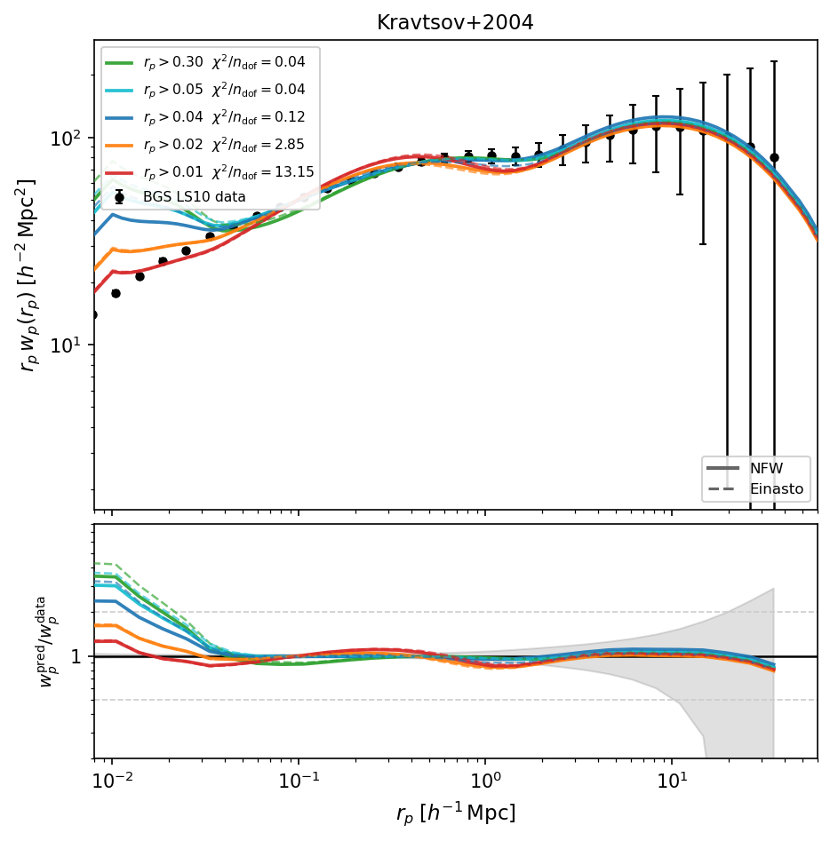
Best-fit \(w_p(r_p)\) for Kravtsov+2004 at all scale cuts. Solid = NFW; dashed = Einasto. Colours: green = \(r_p>0.30\), cyan = \(r_p>0.05\), blue = \(r_p>0.04\), orange = \(r_p>0.02\), red = \(r_p>0.01\).

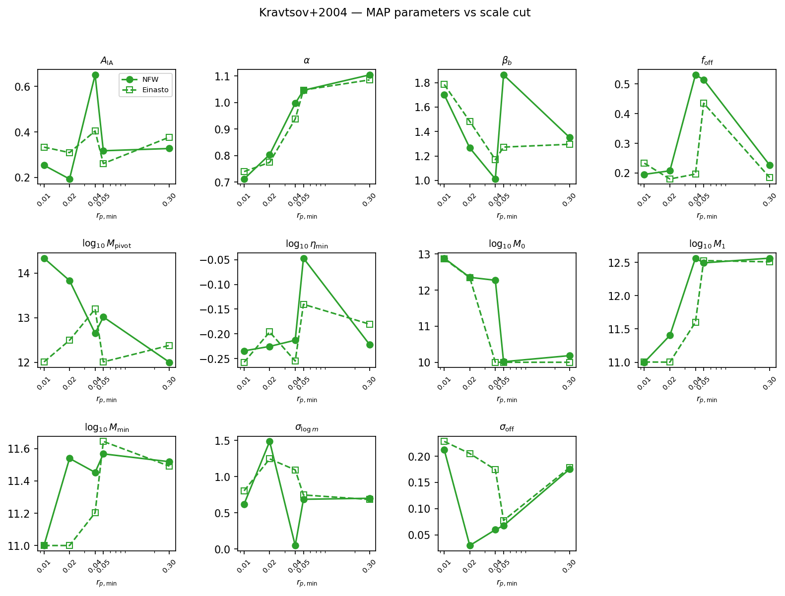
MAP parameter values vs minimum scale \(r_{p,\rm min}\) for Kravtsov+2004. Filled circles / solid = NFW; open circles / dashed = Einasto.

NFW best-fit parameters

Parameter	\(r_p>0.30\)	\(r_p>0.05\)	\(r_p>0.04\)	\(r_p>0.02\)	\(r_p>0.01\)
\(A_{\rm IA}\)	0.327	0.317	0.65	0.193	0.254
\(\alpha\)	1.1	1.05	0.997	0.804	0.711
\(\beta_b\)	1.35	1.86	1.01	1.27	1.7
\(f_{\rm off}\)	0.226	0.514	0.53	0.208	0.196
\(\log_{10}M_{\rm pivot}\)	12	13	12.6	13.8	14.3
\(\log_{10}\eta_{\rm min}\)	-0.221	-0.047	-0.213	-0.225	-0.234
\(\log_{10}M_0\)	10.2	10	12.3	12.4	12.9
\(\log_{10}M_1\)	12.6	12.5	12.6	11.4	11
\(\log_{10}M_{\rm min}\)	11.5	11.6	11.5	11.5	11
\(\sigma_{\log m}\)	0.702	0.688	0.05	1.49	0.622
\(\sigma_{\rm off}\)	0.175	0.0676	0.0596	0.0295	0.213

Einasto best-fit parameters

Parameter	\(r_p>0.30\)	\(r_p>0.05\)	\(r_p>0.04\)	\(r_p>0.02\)	\(r_p>0.01\)
\(A_{\rm IA}\)	0.377	0.261	0.404	0.309	0.333
\(\alpha\)	1.09	1.05	0.938	0.774	0.739
\(\beta_b\)	1.3	1.27	1.17	1.48	1.78
\(f_{\rm off}\)	0.185	0.435	0.197	0.18	0.233
\(\log_{10}M_{\rm pivot}\)	12.4	12	13.2	12.5	12
\(\log_{10}\eta_{\rm min}\)	-0.18	-0.14	-0.255	-0.196	-0.257
\(\log_{10}M_0\)	10	10	10	12.3	12.9
\(\log_{10}M_1\)	12.5	12.5	11.6	11	11
\(\log_{10}M_{\rm min}\)	11.5	11.6	11.2	11	11
\(\sigma_{\log m}\)	0.686	0.748	1.09	1.25	0.806
\(\sigma_{\rm off}\)	0.178	0.0773	0.174	0.205	0.228

Zu & Mandelbaum 2015

\(\chi^2/n_{\rm dof}\) — zu_mandelbaum15

Profile	\(r_p>0.30\)	\(r_p>0.05\)	\(r_p>0.04\)	\(r_p>0.02\)	\(r_p>0.01\)
NFW	0.07	0.22	0.64	2.21	19.22
EINASTO	0.06	0.31	0.59	2.83	22.95

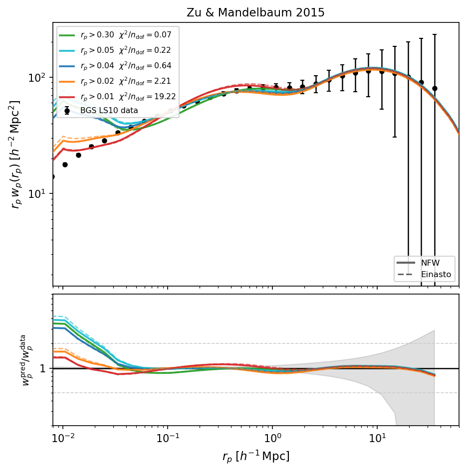
Best-fit \(w_p(r_p)\) for Zu & Mandelbaum 2015 at all scale cuts. Solid = NFW; dashed = Einasto. Colours: green = \(r_p>0.30\), cyan = \(r_p>0.05\), blue = \(r_p>0.04\), orange = \(r_p>0.02\), red = \(r_p>0.01\).

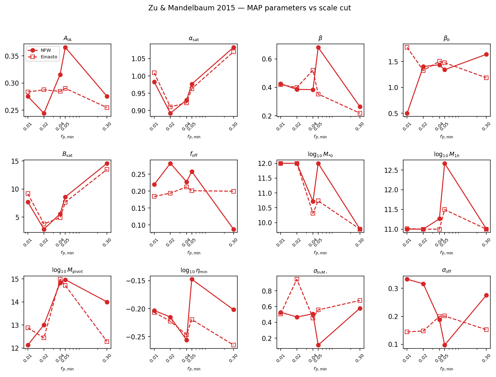
MAP parameter values vs minimum scale \(r_{p,\rm min}\) for Zu & Mandelbaum 2015. Filled circles / solid = NFW; open circles / dashed = Einasto.

NFW best-fit parameters

Parameter	\(r_p>0.30\)	\(r_p>0.05\)	\(r_p>0.04\)	\(r_p>0.02\)	\(r_p>0.01\)
\(A_{\rm IA}\)	0.275	0.366	0.316	0.244	0.275
\(\alpha_{\rm sat}\)	1.08	0.976	0.93	0.892	0.983
\(\beta\)	0.264	0.681	0.384	0.386	0.426
\(\beta_b\)	1.64	1.34	1.44	1.4	0.5
\(B_{\rm sat}\)	14.6	8.58	5.57	2.85	7.68
\(f_{\rm off}\)	0.0875	0.258	0.227	0.282	0.219
\(\log_{10}M_{*0}\)	9.78	12	10.7	12	12
\(\log_{10}M_{1h}\)	11	12.7	11.3	11	11
\(\log_{10}M_{\rm pivot}\)	14	15	14.8	13	12.1
\(\log_{10}\eta_{\rm min}\)	-0.202	-0.148	-0.256	-0.215	-0.203
\(\sigma_{\ln M_*}\)	0.58	0.112	0.508	0.468	0.528
\(\sigma_{\rm off}\)	0.276	0.0975	0.189	0.316	0.333

Einasto best-fit parameters

Parameter	\(r_p>0.30\)	\(r_p>0.05\)	\(r_p>0.04\)	\(r_p>0.02\)	\(r_p>0.01\)
\(A_{\rm IA}\)	0.255	0.29	0.285	0.287	0.284
\(\alpha_{\rm sat}\)	1.07	0.963	0.922	0.91	1.01
\(\beta\)	0.219	0.353	0.521	0.399	0.419
\(\beta_b\)	1.19	1.48	1.51	1.33	1.78
\(B_{\rm sat}\)	13.5	7.65	4.89	3.78	9.17
\(f_{\rm off}\)	0.199	0.201	0.212	0.194	0.184
\(\log_{10}M_{*0}\)	9.78	10.7	10.3	12	12
\(\log_{10}M_{1h}\)	11	11.5	11	11	11
\(\log_{10}M_{\rm pivot}\)	12.3	14.7	15	12.4	12.9
\(\log_{10}\eta_{\rm min}\)	-0.265	-0.219	-0.246	-0.223	-0.207
\(\sigma_{\ln M_*}\)	0.678	0.558	0.455	0.947	0.508
\(\sigma_{\rm off}\)	0.152	0.201	0.2	0.148	0.145

van Uitert+2016

\(\chi^2/n_{\rm dof}\) — vanuitert16

Profile	\(r_p>0.30\)	\(r_p>0.05\)	\(r_p>0.04\)	\(r_p>0.02\)	\(r_p>0.01\)
NFW	0.11	0.39	0.69	6.22	12.75
EINASTO	0.13	0.36	0.62	3.63	35.05

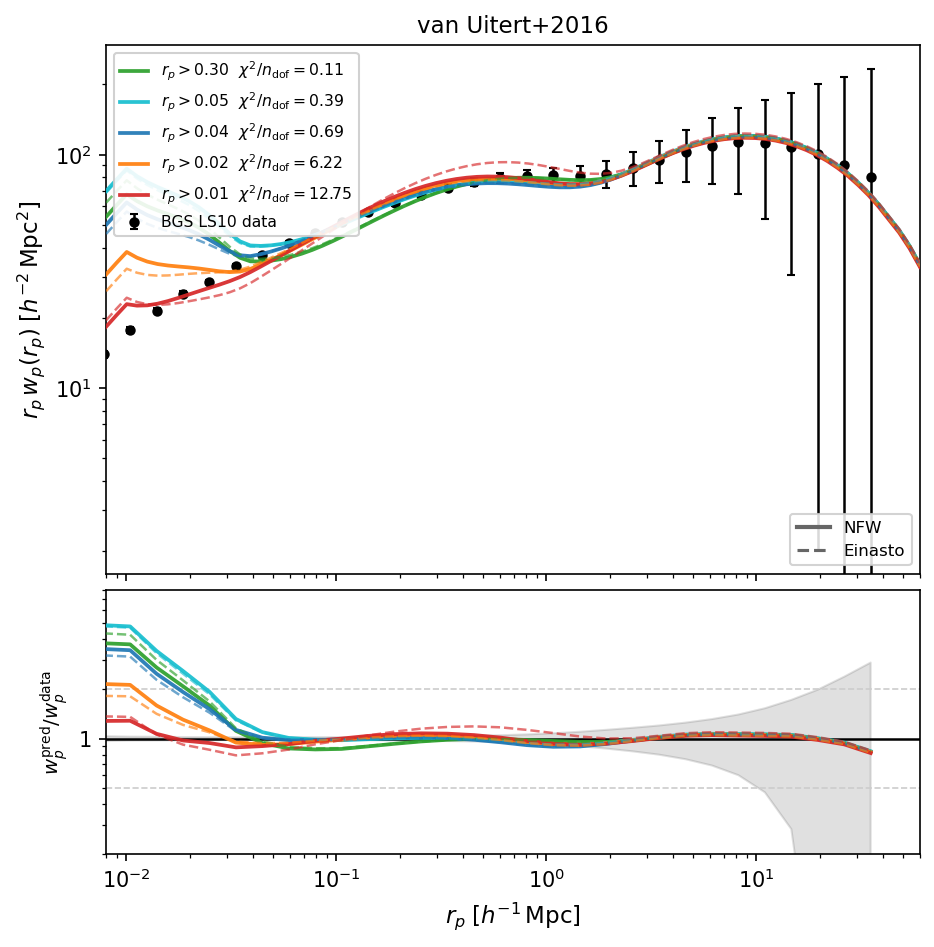
Best-fit \(w_p(r_p)\) for van Uitert+2016 at all scale cuts. Solid = NFW; dashed = Einasto. Colours: green = \(r_p>0.30\), cyan = \(r_p>0.05\), blue = \(r_p>0.04\), orange = \(r_p>0.02\), red = \(r_p>0.01\).

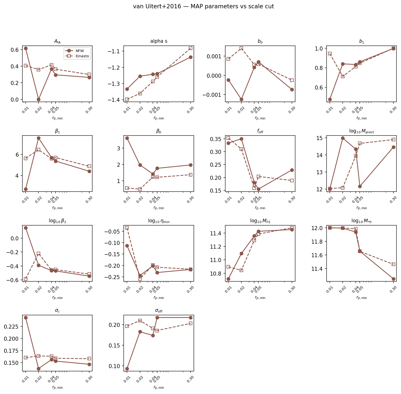
MAP parameter values vs minimum scale \(r_{p,\rm min}\) for van Uitert+2016. Filled circles / solid = NFW; open circles / dashed = Einasto.

NFW best-fit parameters

Parameter	\(r_p>0.30\)	\(r_p>0.05\)	\(r_p>0.04\)	\(r_p>0.02\)	\(r_p>0.01\)
\(A_{\rm IA}\)	0.264	0.295	0.367	3.76e-07	0.615
alpha_s	-1.14	-1.24	-1.24	-1.25	-1.33
\(b_0\)	-0.000742	0.000705	0.000416	-0.00125	-0.000235
\(b_1\)	0.997	0.861	0.833	0.84	0.478
\(\beta_1\)	4.41	5.37	5.7	7.56	2.71
\(\beta_b\)	1.97	1.77	1.43	1.98	3.62
\(f_{\rm off}\)	0.229	0.155	0.18	0.35	0.333
\(\log_{10}M_{\rm pivot}\)	14.5	12.2	14.3	15	12
\(\log_{10}\beta_2\)	-0.546	-0.471	-0.466	-0.391	0.147
\(\log_{10}\eta_{\rm min}\)	-0.218	-0.231	-0.202	-0.244	-0.113
\(\log_{10}M_{h1}\)	11.5	11.4	11.4	11.1	10.7
\(\log_{10}M_{*0}\)	11.3	11.7	11.9	12	12
\(\sigma_c\)	0.147	0.153	0.156	0.138	0.244
\(\sigma_{\rm off}\)	0.217	0.217	0.174	0.183	0.0936

Einasto best-fit parameters

Parameter	\(r_p>0.30\)	\(r_p>0.05\)	\(r_p>0.04\)	\(r_p>0.02\)	\(r_p>0.01\)
\(A_{\rm IA}\)	0.3	0.363	0.415	0.359	0.407
alpha_s	-1.08	-1.26	-1.29	-1.36	-1.4
\(b_0\)	-0.000252	0.000588	0.000563	0.00141	0.000856
\(b_1\)	0.998	0.847	0.812	0.711	0.945
\(\beta_1\)	4.87	5.7	5.59	6.45	5.63
\(\beta_b\)	1.38	1.22	1.23	0.5	0.56
\(f_{\rm off}\)	0.188	0.204	0.159	0.31	0.353
\(\log_{10}M_{\rm pivot}\)	14.9	14.7	13.9	12.1	12
\(\log_{10}\beta_2\)	-0.517	-0.452	-0.459	-0.221	-0.584
\(\log_{10}\eta_{\rm min}\)	-0.216	-0.208	-0.199	-0.259	-0.0347
\(\log_{10}M_{h1}\)	11.5	11.4	11.3	10.8	10.9
\(\log_{10}M_{*0}\)	11.5	11.7	12	12	12
\(\sigma_c\)	0.158	0.159	0.163	0.164	0.16
\(\sigma_{\rm off}\)	0.203	0.186	0.191	0.21	0.196

Zacharegkas+2025

\(\chi^2/n_{\rm dof}\) — zacharegkas25

Profile	\(r_p>0.30\)	\(r_p>0.05\)	\(r_p>0.04\)	\(r_p>0.02\)	\(r_p>0.01\)
NFW	0.11	0.22	0.38	3.14	23.81
EINASTO	0.10	0.10	0.57	2.54	29.27

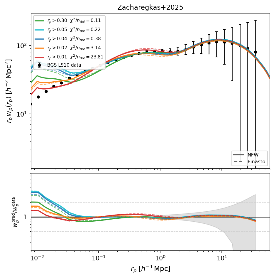
Best-fit \(w_p(r_p)\) for Zacharegkas+2025 at all scale cuts. Solid = NFW; dashed = Einasto. Colours: green = \(r_p>0.30\), cyan = \(r_p>0.05\), blue = \(r_p>0.04\), orange = \(r_p>0.02\), red = \(r_p>0.01\).

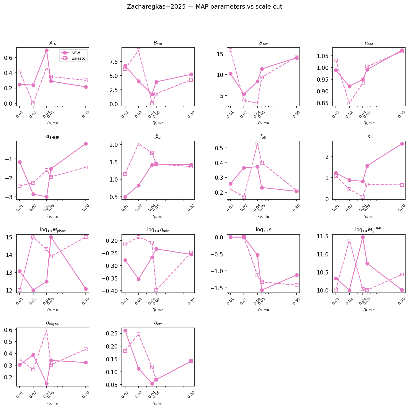
MAP parameter values vs minimum scale \(r_{p,\rm min}\) for Zacharegkas+2025. Filled circles / solid = NFW; open circles / dashed = Einasto.

NFW best-fit parameters

Parameter	\(r_p>0.30\)	\(r_p>0.05\)	\(r_p>0.04\)	\(r_p>0.02\)	\(r_p>0.01\)
\(A_{\rm IA}\)	0.216	0.289	0.694	0.241	0.247
\(B_{\rm cut}\)	5.24	3.91	1.73	4.02	6.78
\(B_{\rm sat}\)	14.1	11.4	8.39	5.29	10.3
\(\alpha_{\rm sat}\)	1.07	0.991	0.949	0.921	0.989
\(\alpha_{\rm SHMR}\)	-0.203	-1.52	-2.99	-2.86	-1.16
\(\beta_b\)	1.42	1.43	1.42	0.825	0.5
\(f_{\rm off}\)	0.207	0.233	0.372	0.366	0.259
\(\kappa\)	2.61	1.56	0.824	0.896	1.22
\(\log_{10}M_{\rm pivot}\)	12.1	15	12.5	12	13.1
\(\log_{10}\eta_{\rm min}\)	-0.256	-0.234	-0.267	-0.354	-0.278
\(\log_{10}\varepsilon\)	-1.12	-1.57	-0.528	-7.77e-05	-0.00234
\(\log_{10}M_1^{\rm SHMR}\)	10	10.7	11.5	10	10.3
\(\sigma_{\log M_*}\)	0.323	0.341	0.147	0.387	0.304
\(\sigma_{\rm off}\)	0.141	0.07	0.0546	0.113	0.261

Einasto best-fit parameters

Parameter	\(r_p>0.30\)	\(r_p>0.05\)	\(r_p>0.04\)	\(r_p>0.02\)	\(r_p>0.01\)
\(A_{\rm IA}\)	0.301	0.35	0.47	1.43e-06	0.419
\(B_{\rm cut}\)	4.25	1.82	0.1	9.5	6.22
\(B_{\rm sat}\)	14.3	9.37	3.12	3.8	15.9
\(\alpha_{\rm sat}\)	1.07	1	0.935	0.848	1.03
\(\alpha_{\rm SHMR}\)	-1.45	-1.95	-1.59	-2.27	-2.42
\(\beta_b\)	1.37	1.43	1.76	2.02	1.15
\(f_{\rm off}\)	0.213	0.4	0.528	0.171	0.221
\(\kappa\)	0.661	0.675	0.1	0.455	1.08
\(\log_{10}M_{\rm pivot}\)	15	13.9	14.3	15	12
\(\log_{10}\eta_{\rm min}\)	-0.248	-0.398	-0.208	-0.186	-0.215
\(\log_{10}\varepsilon\)	-1.42	-1.32	-1.13	-2.83e-06	-0.0046
\(\log_{10}M_1^{\rm SHMR}\)	10.4	10	10	11.4	10
\(\sigma_{\log M_*}\)	0.435	0.303	0.593	0.266	0.348
\(\sigma_{\rm off}\)	0.141	0.0699	0.117	0.247	0.182

Output files

All results are stored under hod_mod/results/bgs_multiprobe/. Directory naming convention:

mstar{MSTAR}_{PROBES}_{MODEL}_{PROFILE}_rp{RPMIN_mmh}[_fcosmo][_fcalib][_sext]/

where rp{RPMIN_mmh} encodes \(r_{p,\rm min}\) in integer milli-\(h^{-1}\,\text{Mpc}\) (e.g. rp020 for 0.02 \(h^{-1}\,\text{Mpc}\)).

Each subdirectory contains:

map_result.json     — best-fit params, χ², ndof, all run metadata
flatchain.npz       — emcee posterior samples (MCMC runs only)

The figure script is at scripts/fitting/bgs_ls10/plot_wp_survey.py.

References

• More et al. 2015 — arXiv:1407.1856

• Zheng et al. 2007 — arXiv:astro-ph/0703457

• Kravtsov et al. 2004 — ApJ 609, 35

• Zu & Mandelbaum 2015 — arXiv:1505.02781

• van Uitert et al. 2016 — arXiv:1601.06791

• Zacharegkas & Chang et al. 2025 — arXiv:2506.22367

• Johnston et al. 2007 — arXiv:0709.4193

• Bridle & King 2007 — arXiv:0705.0166

• FLAMINGO — arXiv:2510.25419

• DESI BGS — Hahn et al. 2023 arXiv:2208.08512