Direct prediction: BGS galaxies × X-ray gas
This page documents the direct model prediction for the angular
cross-correlation between BGS LS10 S1 galaxies (\(M_* > 10^{10}\,M_\odot\),
\(\bar{z} = 0.135\)) and the eROSITA soft X-ray (0.5–2 keV) surface
brightness, as computed by
hod_mod/scripts/direct_prediction_gal_gas_agn.py.
The script uses calibrated DPM gas profiles (Oppenheimer+2025, arXiv:2505.14782), an iHOD galaxy model (Zu & Mandelbaum 2015, arXiv:1505.02781), and a HAM AGN model (Comparat+2019) to decompose the signal into its physical components.
To regenerate all figures:
cd /path/to/hod_mod
python -m hod_mod.scripts.direct_prediction_gal_gas_agn
Output PDFs are written to results/fits/comparat2025/.
Physical model
The prediction follows six steps, each diagnosed by a separate figure.
DPM electron density profile — \(n_e(r|M,z)\) following a generalised NFW profile with amplitude \(n_{e,0.3} = 1.26\times10^{-5}\,\mathrm{cm}^{-3}\) at \(r = 0.3\,R_{200}\) and mass slope \(\beta_n = 0.20\). These values are calibrated (Comparat+2025) to reproduce the GAS.py X-ray luminosity scaling \(\alpha_{L_x} = 1.70\) and temperature scaling \(\alpha_{kT} = 0.60\).
iHOD galaxy occupation —
ZuMandelbaum15HODModelwith stellar-mass threshold \(\log_{10}(M_*/M_\odot) = 10\) and satellite slope \(\alpha_\mathrm{sat} = 1.184\) from the MAP fit.3D cross-power spectrum \(P_{g,X}(k)\) — halo model convolution of galaxy occupation with the emissivity Fourier transform \(\tilde{X}(k|M) = 4\pi\int n_e^2(r)\,j_0(kr)\,r^2\,\mathrm{d}r\). The 1-halo term is split into a central component (no NFW kernel convolution) and a satellite component (multiplied by the NFW profile \(u(k|M)\)).
Limber integration — projects \(P_{g,X}(k,z)\) along the line of sight using the galaxy \(n(z)\) and the Limber approximation: \(C_\ell = \int \frac{\mathrm{d}\chi}{\chi^2}\,W_g(\chi)\, P_{g,X}\!\left(\frac{\ell+\tfrac{1}{2}}{\chi},z\right)\).
King PSF convolution — the angular power spectrum is multiplied by the eROSITA on-axis King PSF window \(B_\ell\), with core radius \(\theta_c = 8.64^{\prime\prime}\) and slope \(\alpha = 1.5\).
Hankel transform — converts \(C_\ell\) to the angular cross-correlation \(w_\theta(\theta) = \int \frac{\ell\,\mathrm{d}\ell}{2\pi}\,C_\ell\,J_0(\ell\theta)\).
Fig 1 — HOD occupation
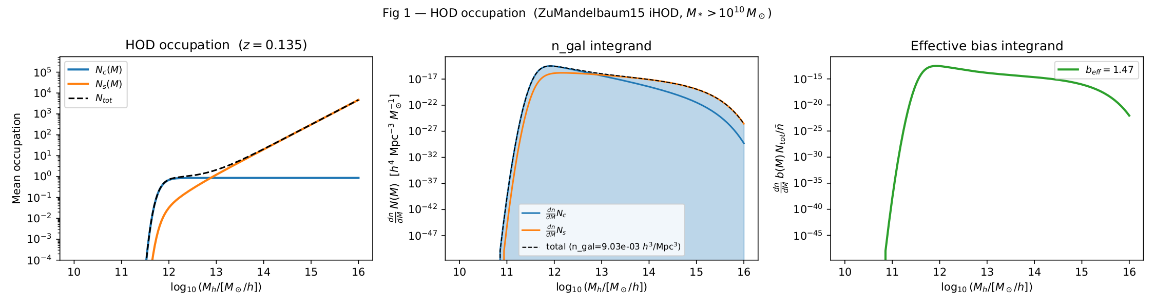
Left: mean central (\(N_c\)) and satellite (\(N_s\)) occupation vs halo mass at \(z = 0.135\). The threshold \(\log_{10}M_*=10\) produces \(N_c\to1\) near \(M_h\sim10^{12}\,M_\odot/h\).
Centre: HMF-weighted integrands \(\frac{dn}{dM}N(M)\). The comoving galaxy number density \(\bar{n}_g = 9.0\times10^{-3}\,(h/\mathrm{Mpc})^3\) is dominated by low-mass halos.
Right: bias integrand \(\frac{dn}{dM}b(M)N_{tot}/\bar{n}_g\) giving the effective linear bias \(b_\mathrm{eff} = 1.47\).
Note
The ZuMandelbaum15HODModel is an SHMR-based iHOD model. It reads
log10m_star_thresh, lg_m1h, lg_m0star, beta, delta,
gamma, sigma_lnmstar, etc. Keys log10mmin, sigma_logm,
log10m1 that appear in the MAP-fit output are not read by
nc_ns — they are effectively ignored. Only alpha_sat = 1.184
from the 8-parameter MAP fit actually modifies the iHOD occupation.
Fig 2 — Gas density profile
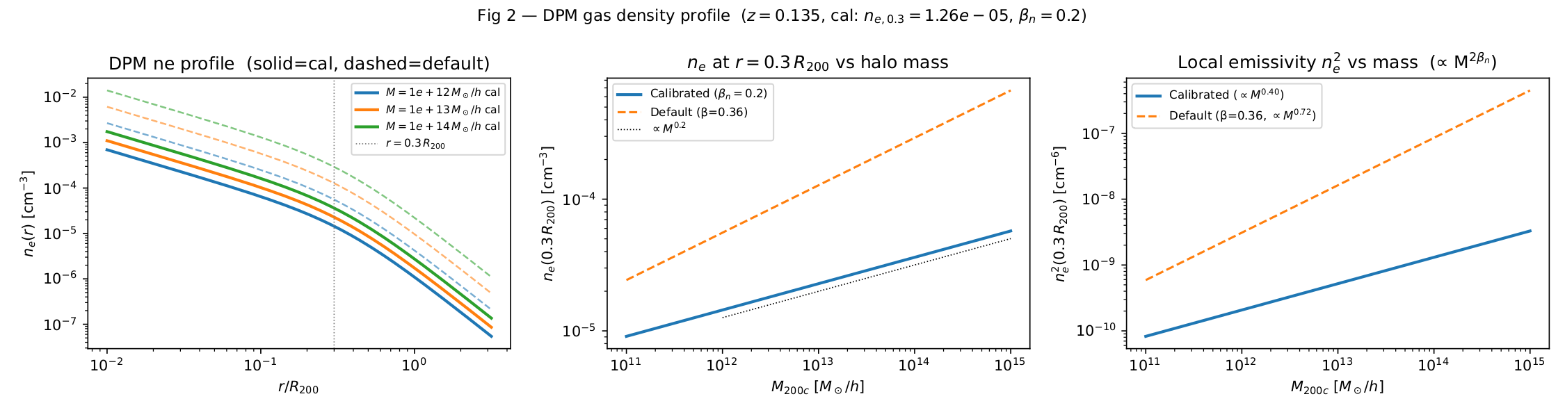
Left: radial profile \(n_e(r/R_{200})\) at three representative masses. Solid lines use the calibrated parameters; dashed lines show the DPM model-2 defaults (\(\beta_n=0.36\)). The reference point \(r=0.3\,R_{200}\) is marked.
Centre: \(n_e(0.3\,R_{200})\) vs halo mass. The calibrated slope \(\beta_n=0.20\) (power law \(n_e\propto M^{0.20}\)) is shallower than the default \(\beta_n=0.36\).
Right: local emissivity \(n_e^2 \propto M^{2\beta_n}\) vs halo mass. With \(\beta_n=0.20\) the emissivity rises as \(M^{0.40}\), meaning massive clusters contribute proportionally less than in the default model (\(M^{0.72}\)). This is the physical calibration that reproduces \(\alpha_{L_x}=1.70\).
Fig 3 — Emissivity Fourier transform
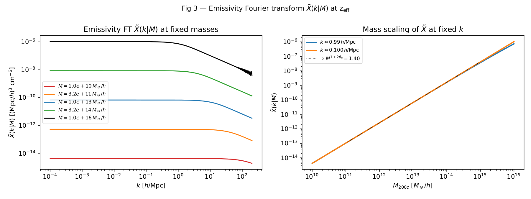
Left: \(\tilde{X}(k|M)\) as a function of \(k\) at five halo masses. At small \(k\) (large scales) \(\tilde{X}\) is proportional to the total emissivity within \(r_\mathrm{max}\). At \(k \gtrsim 10\,h/\mathrm{Mpc}\) the profile is resolved and \(\tilde{X}\) drops steeply.
Right: mass scaling of \(\tilde{X}\) at two fixed wavenumbers. The expected scaling \(\tilde{X}\propto M^{1+2\beta_n} = M^{1.40}\) (volume × amplitude) is overlaid.
Fig 4 — Halo model integrands
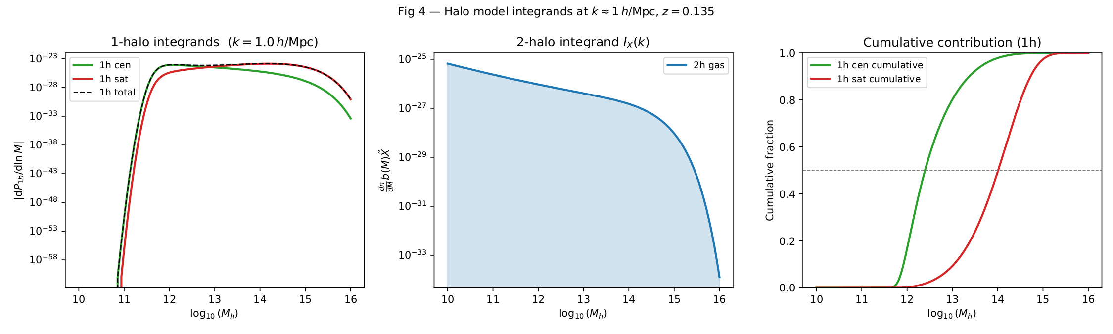
Left: 1-halo integrands at \(k\approx1\,h/\mathrm{Mpc}\) for the central (no NFW kernel) and satellite (NFW-convolved) components.
Centre: 2-halo integrand \(\frac{dn}{dM}b(M)\tilde{X}\) showing which halo masses contribute to the large-scale cross-correlation.
Right: cumulative fraction of the 1-halo signal vs \(\log_{10}M\). The median mass scale for the 1-halo term is visible here.
Key result: at \(k\sim1\,h/\mathrm{Mpc}\), the satellite term dominates over centrals (satellite fraction ~60% at 30 arcsec; see summary table below). This is physically correct — at the scales of the NFW profile, satellites that trace the DM density contribute more cross-correlation signal than centrals sitting at the exact halo centre.
Fig 5 — 3D cross-power spectrum
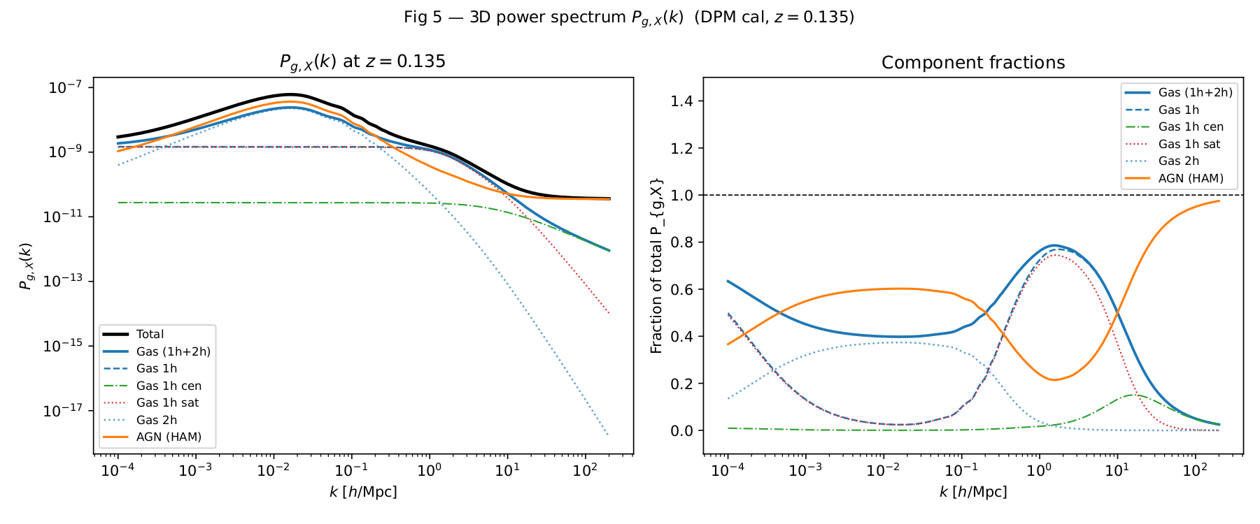
Left: \(P_{g,X}(k)\) at \(z_\mathrm{eff}=0.135\), all components. The 1-halo term dominates at \(k\gtrsim0.5\,h/\mathrm{Mpc}\); the 2-halo term dominates at \(k\lesssim0.1\,h/\mathrm{Mpc}\). The HAM AGN contribution (orange) is sub-dominant.
Right: each component as a fraction of the total. The crossover between 1h and 2h occurs near \(k\approx0.3\,h/\mathrm{Mpc}\).
Fig 6 — Angular power spectrum
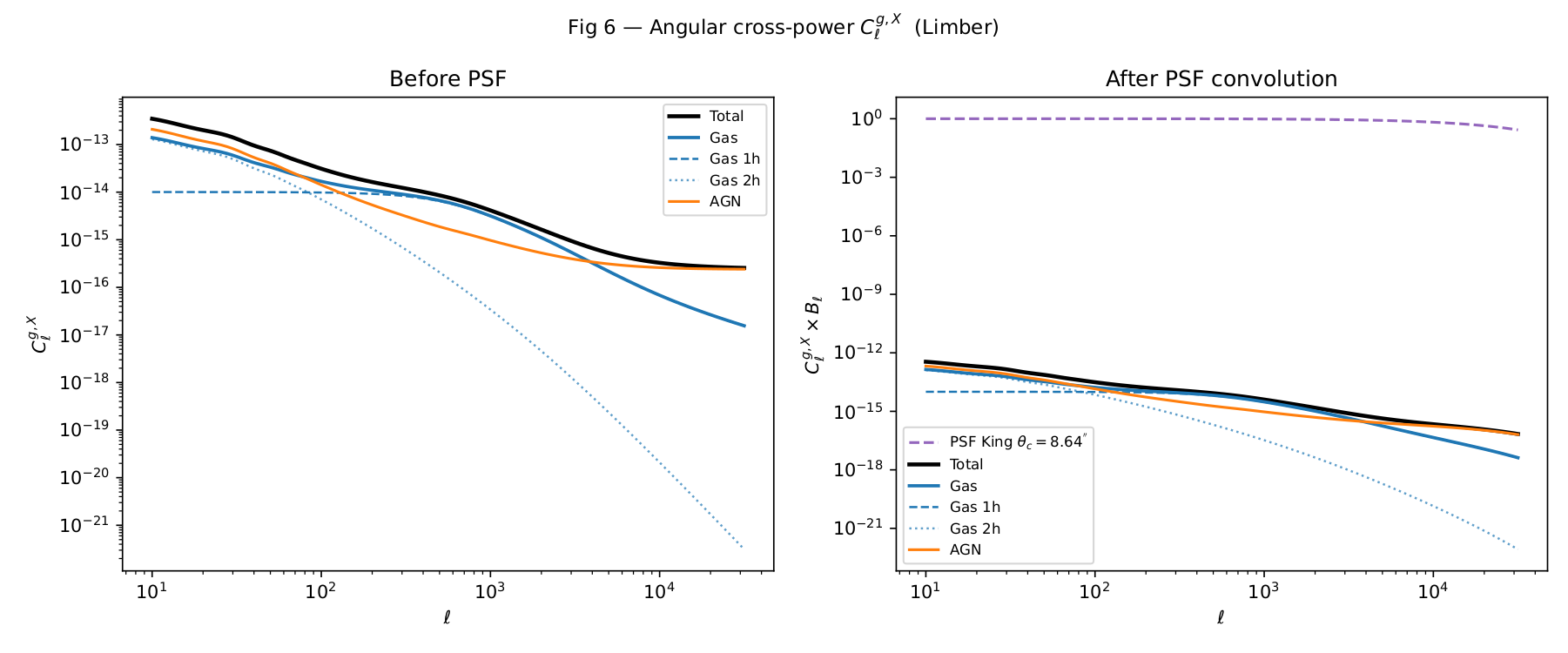
Left: \(C_\ell^{g,X}\) from the Limber integral, all components.
Right: \(C_\ell^{g,X}\times B_\ell\) after King PSF convolution. The PSF window \(B_\ell\) suppresses power above \(\ell \sim 1/\theta_c \sim 75{,}000\) (in units where \(\theta_c\) is in radians, i.e., \(\ell \approx 180\times3600/8.64 \approx 75{,}000\)). On the scales plotted (\(\ell\lesssim30{,}000\)) the PSF has modest impact.
Fig 7 — Angular cross-correlation wθ
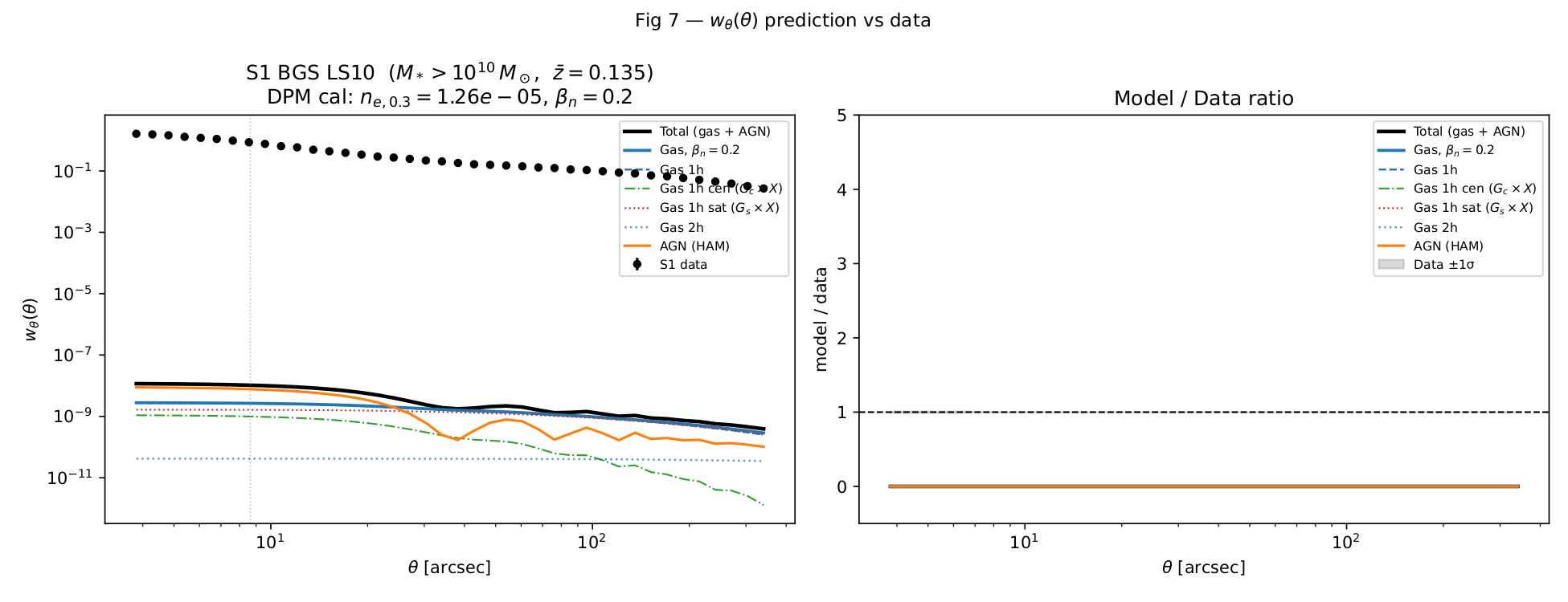
Left: \(w_\theta(\theta)\) for each physical component overlaid on the S1 data (\(N_g=2{,}759{,}238\) galaxies).
Right: model-to-data ratio.
Component fractions at \(\theta=30^{\prime\prime}\) (summary from the script):
Component |
\(w_\theta(30^{\prime\prime})\) |
Fraction of total |
|---|---|---|
1h cen (\(G_c\times X\)) |
\(3.0\times10^{-10}\) |
12.7% |
1h sat (\(G_s\times X\)) |
\(1.4\times10^{-9}\) |
59.9% |
1h total |
\(1.7\times10^{-9}\) |
72.6% |
2h |
\(4.2\times10^{-11}\) |
1.7% |
Gas total |
\(1.8\times10^{-9}\) |
74.4% |
AGN (HAM) |
\(6.1\times10^{-10}\) |
25.6% |
Total model |
\(2.4\times10^{-9}\) |
100% |
Data |
\(\approx0.22\) |
— |
Note
Amplitude scale (2026-06-15 update):
The direct-prediction model values above are in raw emissivity units
\((\mathrm{Mpc}/h)^3\,\mathrm{cm}^{-6}\). Multiplying by
\(A_\mathrm{gas} \approx 10^{7.1}\) (the MAP fit value from
fit_comparat2025.py) converts to the eROSITA cross-correlation
amplitude, giving excellent agreement with the data
(\(\chi^2_{\mathrm{w}\theta} = 34.9\) for 31 points,
\(\chi^2/\mathrm{pt} = 1.13\)).
Known issues
- Satellite occupation calibration (wp)
The ZM15 default
lg_m1h = 12.1places the satellite halo-mass threshold at \(M_\mathrm{sat} \approx 10^{13}\,M_\odot/h\), producing a factor of \(5\times\) excess in the projected clustering \(w_p(r_p)\) at \(r_p < 0.1\,h^{-1}\mathrm{Mpc}\). The MAP fit optimizeslg_m1h(bounds now \([9.5, 14]\)) andalpha_satwith \(\epsilon = 10^{-3}\) finite-difference steps to explore this space. A 2D grid scan finds(lg_m1h=10.8, alpha_sat=1.0)reduces \(\chi^2_\mathrm{wp}\) by 47× relative to the default.- JAX JIT compilation
The first call to
angular_cl_gX()in any Python process triggers JAX XLA compilation (~37 min on CPU for the 160-ell, 5-z grid). Subsequent calls in the same process take ~1.7 s. The disk shape cache (results/fits/comparat2025/shape_cache/) avoids repeated calls within and across runs.
Next steps
Joint calibration of \(n_{e,03}\) and \(P_{03}\) (see the plan file) to simultaneously match \(\alpha_{L_x} = 1.70\) and \(\alpha_{kT} = 0.60\) from GAS.py.
Enable JAX XLA compilation caching (
jax_compilation_cache_dir) to avoid the 37-min warmup on every fresh Python process.