Forward Model Showcase
This page illustrates the full HOD forward-model pipeline for a fiducial
Planck 2018 cosmology (arXiv:1807.06209)
using the Tinker+2008 HMF (arXiv:0803.2706),
the More+2015 HOD (arXiv:1407.1856),
the beyond-linear halo bias correction of Mead & Verde 2021
(arXiv:2011.08858, implemented in
BeyondLinearBiasMead21),
and the NLA intrinsic-alignment model
(arXiv:0705.0166).
These figures are pre-generated by a sensitivity-study driver that exercises the
public API documented on this page, and ship with the documentation under
docs/_images/.
Pipeline Summary
The table below identifies which pipeline feature each HOD model variant supports. ✓ = supported; — = not applicable / uses a different mechanism. Abbreviations: Zh07 = Zheng+2007, K04 = Kravtsov+2004, Mo15 = More+2015, ZM15 = Zu & Mandelbaum 2015, VU16 = van Uitert+2016, Za25 = Zacharegkas+2025, Gu18 = Guo+2018 ICSMF, Gu19 = Guo+2019 ICSMF, ZM16Q = ZuMandelbaum16Quenching.
Feature / pipeline step |
Zh07 |
K04 |
Mo15 |
ZM15 |
VU16 |
Za25 |
Gu18 |
Gu19 |
ZM16Q |
|---|---|---|---|---|---|---|---|---|---|
\(P_{\rm lin}\) → HMF → \(b(M)\) → \(c(M)\) → \(\tilde{u}(k|M)\) |
✓ |
✓ |
✓ |
✓ |
✓ |
✓ |
✓ |
✓ |
✓ |
\(N_c\) via erfc threshold on halo mass |
✓ |
✓ |
✓ |
— |
— |
— |
— |
— |
— |
\(N_c\) via SHMR + stellar-mass threshold |
— |
— |
— |
✓ |
— |
✓ |
— |
— |
— |
\(N_c\) via SHMR + stellar-mass bin (CSMF) |
— |
— |
— |
— |
✓ |
— |
✓ |
✓ |
— |
\(N_s\) via power law \((M-M_0)/M_1\) |
✓ |
— |
✓ |
— |
— |
— |
— |
— |
— |
\(N_s\) via \(N_c\,(M/M_1)^\alpha\exp(-M_0/M)\) |
— |
✓ |
— |
✓ |
— |
✓ |
✓ |
✓ |
— |
\(N_s\) via CSMF Schechter integral |
— |
— |
— |
— |
✓ |
— |
✓ |
✓ |
— |
Satellite cut-off \(\kappa M_{\min}\) |
— |
— |
✓ |
— |
— |
— |
— |
— |
— |
Incompleteness correction \(f_{\rm inc}(M)\) |
— |
— |
✓ |
— |
— |
— |
✓ |
✓ |
— |
Mass-dependent scatter \(\sigma_{\ln M_*}(M)\) |
— |
— |
— |
✓ |
— |
— |
— |
— |
— |
Red/blue quenching fractions \(f_{\rm red}(M)\) |
— |
— |
— |
— |
— |
— |
— |
✓ |
✓ |
Off-centering \(W_{\rm off}(k)\) (Johnston+2007) |
✓ |
✓ |
✓ |
✓ |
✓ |
✓ |
✓ |
✓ |
✓ |
NLA intrinsic-alignment correction |
✓ |
✓ |
✓ |
✓ |
✓ |
✓ |
✓ |
✓ |
✓ |
Beyond-linear bias \(\beta^{\rm NL}(k,\nu_1,\nu_2)\) (Mead & Verde 2021) |
✓ |
✓ |
✓ |
✓ |
✓ |
✓ |
✓ |
✓ |
✓ |
\(P_{gg},\,P_{gm}\) → \(w_p(r_p),\,\Delta\Sigma(R)\) |
✓ |
✓ |
✓ |
✓ |
✓ |
✓ |
✓ |
✓ |
✓ |
The cosmological steps shared by all models are:
LinearPowerSpectrum .pk_linear() (CAMB) →
HaloMassFunction .dndm() / .bias() →
BeyondLinearBiasMead21 (beyond-linear \(\beta^{\rm NL}\)) →
HaloProfile .concentration() / nfw_uk() / einasto_uk() →
hod_mod.connection.hod .nc_ns() →
wp() /
delta_sigma().
1. Linear Matter Power Spectrum
The linear matter power spectrum \(P_{\rm lin}(k,z)\) is computed via CAMB (arXiv:astro-ph/9911177) at the BGS effective redshift \(z = 0.14\). Two additional curves show the \(\pm 3\sigma\) S8 variation from Planck 2018 (S8 = 0.832 ± 0.013):
since \(P_{\rm lin} \propto A_s \propto \sigma_8^2\) at fixed shape.
where \(T(k)\) is the matter transfer function (Lewis, Challinor & Lasenby 2000) and \(D(z)\) the linear growth factor. The fiducial parameters are the Planck 2018 best-fit: \(h=0.6736\), \(\Omega_m=0.3100\), \(n_s=0.9649\), \(\ln(10^{10}A_s)=3.044\).
References: Lewis, Challinor & Lasenby 2000 (arXiv:astro-ph/9911177); Planck 2018 (arXiv:1807.06209).
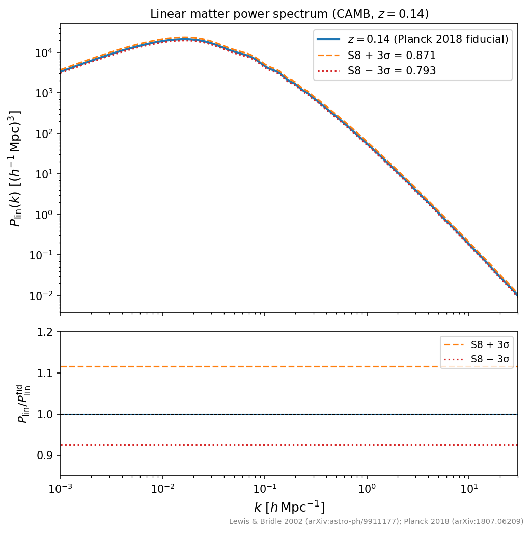
Linear matter power spectrum \(P_{\rm lin}(k)\) at \(z=0.14\) with \(\pm 3\sigma\) S8 variation (Planck 2018).
2. Non-Linear Matter Power Spectrum
On scales \(k \gtrsim 0.1\,h\,{\rm Mpc}^{-1}\) gravitational collapse drives
the power spectrum above the linear prediction.
The ratio \(P_{\rm nl}/P_{\rm lin}\) captures the 1-halo boost, mode coupling,
and quasi-linear BAO damping. The 1-halo + 2-halo decomposition in
FullHaloModelPrediction uses
\(P_{\rm lin}\) for the 2-halo term and mass-integrated NFW profiles for the
1-halo term — the total galaxy power spectrum does not directly use
\(P_{\rm nl}\), but it is available for diagnostic comparisons and as an
optional non-linear 2-halo term (nl_2halo=True).
Four backends are implemented in hod_mod.core.nonlinear:
Class |
Reference |
Valid range |
Notes |
|---|---|---|---|
|
Sanchez 2025 (arXiv:2511.13826) |
\(k \in [0.006, 2]\,{\rm Mpc}^{-1}\) |
Emulator; JAX-native |
|
Chen et al. 2025 CEmulator v2.0 |
\(k \in [0.005, 10]\,h\,{\rm Mpc}^{-1}\), \(z \in [0, 3]\) |
Requires |
|
Mead et al. 2020 (arXiv:2009.01858) |
\(k \in [10^{-4}, 20]\,h\,{\rm Mpc}^{-1}\) |
CAMB HMcode-2020 (default); also |
|
Brieden et al. 2025 (arXiv:2508.10902) |
\(k \in [10^{-2}, 10]\,h\,{\rm Mpc}^{-1}\) |
Web-Halo Model; zero free parameters; requires WHM-CAMB fork
( |
All backends share the same interface and can be wrapped with
CachedPkNonlinear for MCMC hot loops:
from hod_mod.core.nonlinear import HALOFITSpectrum, WHMSpectrum, CachedPkNonlinear

# Standard CAMB HMcode-2020
pk_nl = CachedPkNonlinear(HALOFITSpectrum(halofit_version="mead2020"))

# WHM (requires WHM-CAMB fork)
pk_nl = CachedPkNonlinear(WHMSpectrum(whm_version="brieden2023"))

# Pass to FullHaloModelPrediction for a non-linear 2-halo term
pred = FullHaloModelPrediction(pk_lin, hod, profile, pk_nl=pk_nl, nl_2halo=True)
Figure generated by
hod_mod/scripts/cosmology/plot_nonlinear_power_spectrum.py.
References: Aletheia (arXiv:2511.13826); Mead et al. 2020 HMcode (arXiv:2009.01858); Takahashi et al. 2012 (arXiv:1208.2701); Smith et al. 2003 HALOFIT (arXiv:astro-ph/0207664); Brieden et al. 2025 WHM (arXiv:2508.10902).
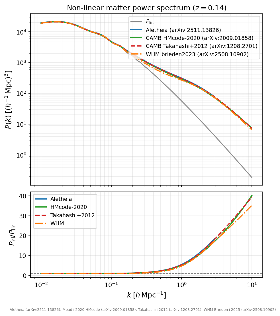
Non-linear matter power spectrum \(P_{\rm nl}(k)\) at \(z=0.14\) (top) and boost ratio \(P_{\rm nl}/P_{\rm lin}\) (bottom): Aletheia emulator, CAMB HMcode-2020, and CAMB Takahashi+2012 backends. WHM (Brieden+2025) shown once WHM-CAMB is installed.
3. Halo Mass Function and Linear Bias
The comoving number density of halos per unit mass interval is computed by
dndm():
where \(\sigma^2(M)\) is the variance of the linear density field smoothed
on scale \(R = (3M/4\pi\bar{\rho}_m)^{1/3}\), evaluated by
sigma().
The multiplicity function \(f(\sigma)\) follows Tinker et al. 2008
(calibrated to \(\Delta=200m\)):
The large-scale linear bias \(b(M)\) is returned by
bias()
using the peak-background split (Tinker et al. 2010,
arXiv:1001.3162).
Class:
HaloMassFunction
(hod_mod/core/halo_mass_function.py):
from hod_mod.core import HaloMassFunction
from hod_mod.core.power_spectrum import LinearPowerSpectrum, rho_critical_0

pklin  = LinearPowerSpectrum()
rho_m  = rho_critical_0() * theta["Omega_m"]
hmf    = HaloMassFunction(pklin.pk_linear, rho_mean=rho_m, model="tinker08")

dndm   = hmf.dndm(m_h, z, theta)   # [h⁴ M⊙⁻¹ Mpc⁻³]
bias   = hmf.bias(m_h, z, theta)   # dimensionless large-scale bias
sigma  = hmf.sigma(m_h, z, theta)  # RMS density fluctuation σ(M,z)
HaloMassFunction is constructed
with the model keyword selecting the multiplicity function. The 17
implemented models are listed in the table below.
|
Function |
Reference |
|---|---|---|
|
Tinker et al. 2008 (arXiv:0803.2706) |
|
|
Press & Schechter 1974 (ApJ 187, 425) |
|
|
Sheth & Tormen 1999 (arXiv:astro-ph/9901122) |
|
|
Jenkins et al. 2001 (arXiv:astro-ph/0005260) |
|
|
Warren et al. 2006 (arXiv:astro-ph/0506395) |
|
|
Bhattacharya et al. 2011 (arXiv:1005.2239) |
|
|
Crocce et al. 2010 (arXiv:0907.0019) |
|
|
Courtin et al. 2011 (arXiv:1001.3425) |
|
|
Angulo et al. 2012 (arXiv:1203.3216) |
|
|
Watson et al. 2013 (arXiv:1212.0095) |
|
|
Bocquet et al. 2016 (arXiv:1502.07357) |
|
|
Despali et al. 2016 (arXiv:1507.05627) |
|
|
Rodríguez-Puebla et al. 2016 (arXiv:1602.04813) |
|
|
Comparat et al. 2017 (arXiv:1702.01628) |
|
|
Seppi et al. 2020 (arXiv:2006.00818) |
|
|
Yung et al. 2024 |
|
|
Yung et al. 2025 |
Figures generated by hod_mod/scripts/cosmology/plot_hmf_bias.py.
References: Tinker et al. 2008 (arXiv:0803.2706); Tinker et al. 2010 (arXiv:1001.3162).
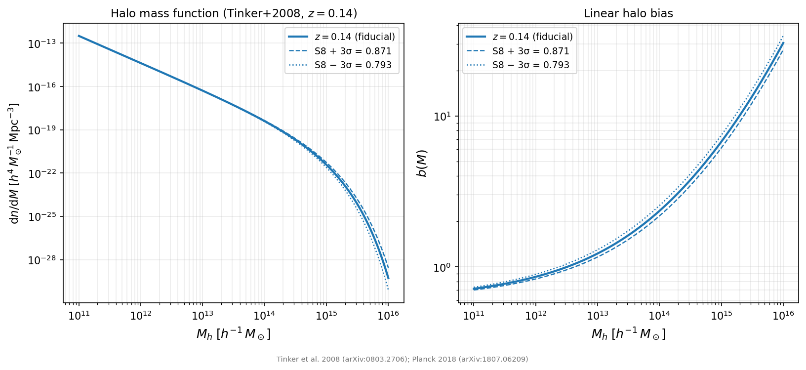
dndm()
and bias()
at \(z=0.14\) with \(\pm 3\sigma\) S8 variation (Tinker+2008/2010).
hod_mod implements 17 analytic multiplicity functions
(fsigma_* in hod_mod.core.halo_mass_function);
the figure below compares six.
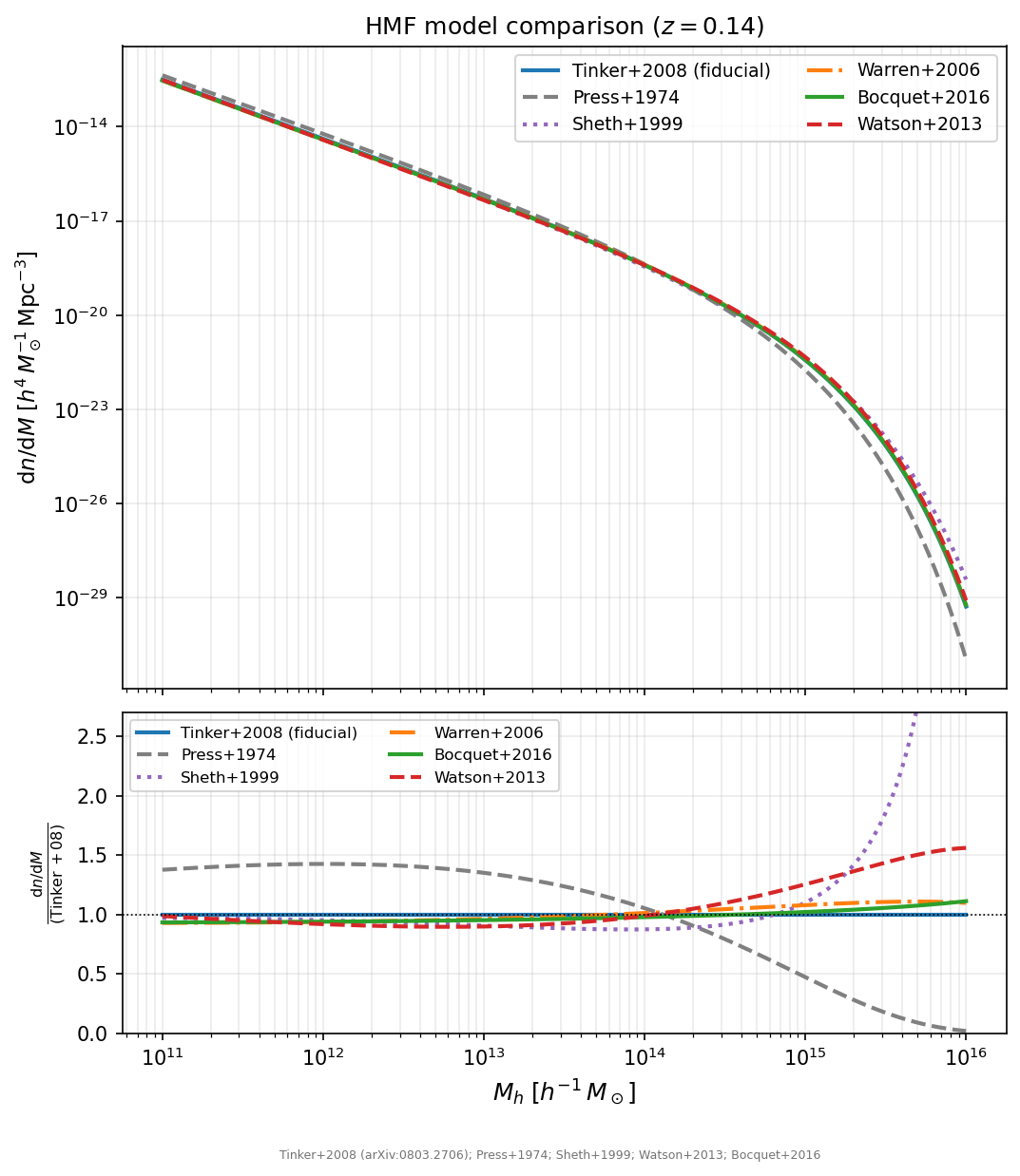
fsigma_tinker08() (fiducial)
vs five alternative multiplicity functions: Press+1974, Sheth+1999,
Warren+2006, Bocquet+2016, Watson+2013.
Bottom panel shows ratio to Tinker+2008.
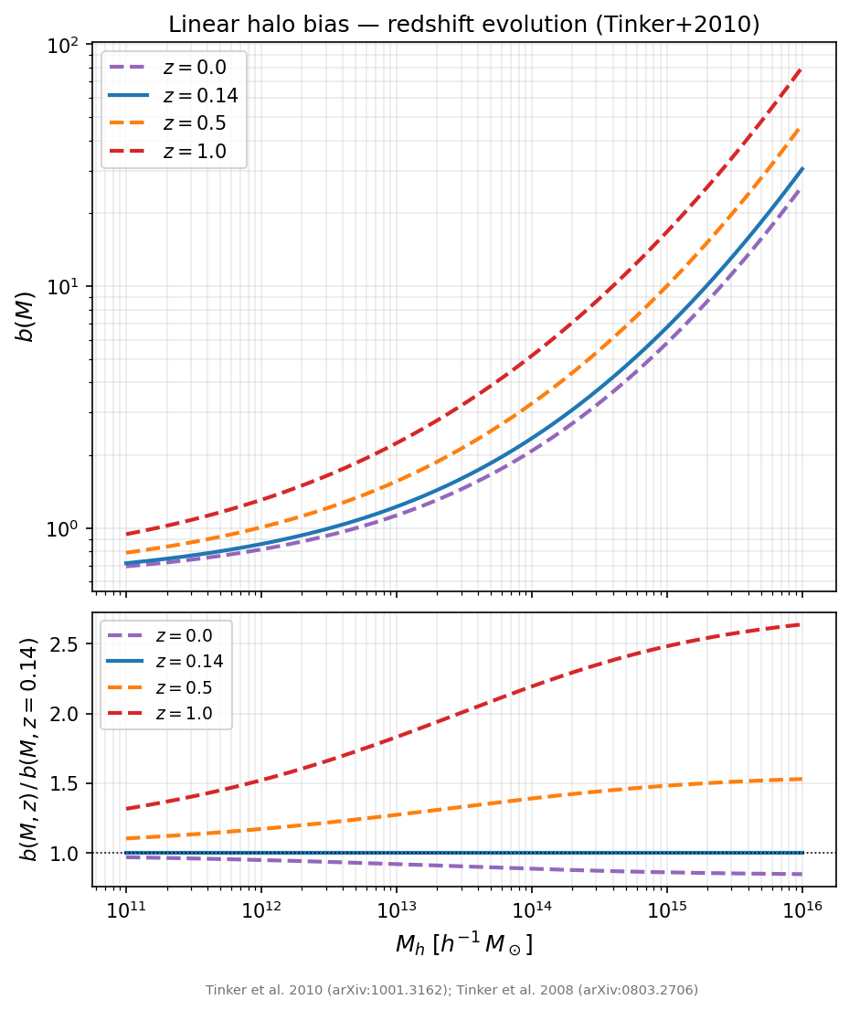
Redshift evolution of
bias()
(Tinker+2010 peak-background split) at \(z = 0, 0.14, 0.5, 1.0\).
Bottom panel shows ratio to \(z=0.14\).
4. Beyond-Linear Halo Bias
At intermediate scales \(k \sim 0.05{-}0.8\,h\,{\rm Mpc}^{-1}\) the large-scale bias approximation \(P_{hh}^{\rm 2h}(k) = b(M)^2 P_{\rm lin}(k)\) underestimates halo–halo clustering relative to N-body simulations. The beyond-linear halo bias (BNL; Mead & Verde 2021, arXiv:2011.08858) quantifies this deviation empirically:
where \(\nu_i = \delta_c/\sigma(M_i)\) is the peak height and \(\beta^{\rm NL}\) is measured from the MultiDark MDR1 N-body simulation (2048³ particles, \(1\,h^{-1}{\rm Gpc}\) box). The data span 8 logarithmically-spaced peak-height bins (\(\nu \in [0.85,\,3.71]\)) and 25 wavenumbers (\(k \in [6.3\times10^{-3},\,0.74]\,h\,{\rm Mpc}^{-1}\)).
Key properties:
\(\beta^{\rm NL}(k\to0,\,\nu_1,\nu_2) = 0\) — recovers linear bias at large scales (\(\beta^{\rm NL} = 0\) for \(k < 6.3\times10^{-3}\,h\,{\rm Mpc}^{-1}\)).
The peak-height parameterisation makes the table approximately cosmology-independent; the same \(z=0\) data applies at any redshift when \(\nu(M,z)\) is computed consistently.
\(\beta^{\rm NL}\) can be positive or negative depending on scale and mass bin.
The additive BNL corrections to the two-halo power spectra are:
These double mass-integrals are evaluated efficiently by projecting the
mass-function weights onto the 8-bin \(\nu\) grid and contracting with the
cached \((N_k \times 8 \times 8)\) \(\beta^{\rm NL}\) table — only an
\(\mathcal{O}(N_k \times N_M \times 8)\) projection per HOD evaluation
is required (see
BeyondLinearBiasMead21).
BNL is the fiducial prescription for the two-halo term in all
hod_mod HOD models. Usage:
from hod_mod.core import BeyondLinearBiasMead21
from hod_mod.observables.clustering import FullHaloModelPrediction

bnl = BeyondLinearBiasMead21()        # loads bundled MDR1 z=0 tables
pred = FullHaloModelPrediction(pk_lin, hod, hp, bnl_model=bnl)
wp = pred.wp(rp, pi_max, z, theta, hod_params)
Passing bnl_model=None reverts to the scale-independent
\(b_{\rm eff}^2\,P_{\rm lin}\) approximation.
Data: Tabulated \(\beta^{\rm NL}\) (snapshot 85 = \(z=0\))
are bundled in hod_mod/data/bnl/; additional snapshots at
\(z = 0.01{-}10\) are available from the BNL repository.
References: Mead & Verde 2021 (arXiv:2011.08858); BNL simulation data: github.com/alexander-mead/BNL.
5. NFW Concentration–Mass Relation
The NFW concentration is defined as
where \(r_{200m}\) is the radius enclosing a mean density 200 times the mean matter density and \(r_s\) is the NFW scale radius. The concentration–mass relation is evaluated via colossus using the Diemer & Joyce 2019 fitting function:
(schematic; see Diemer & Joyce 2019 for the full parametrisation.)
References: Navarro, Frenk & White 1997 (arXiv:astro-ph/9611107); Diemer & Joyce 2019 (arXiv:1809.07326).
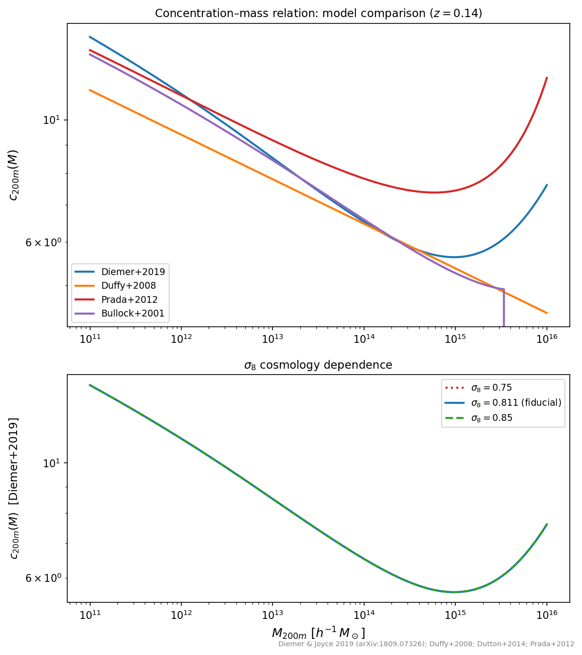
NFW concentration–mass relation \(c_{200m}(M, z)\) from multiple colossus models, including Diemer & Joyce 2019.
6. Halo Profile Fourier Transforms
Two density profile families are implemented: NFW (analytic Fourier transform) and Einasto (numerical transform via Gauss-Legendre quadrature).
NFW profile (Navarro, Frenk & White 1997):
Its Fourier transform normalised to unity at \(k=0\) is (Cooray & Sheth 2002 arXiv:astro-ph/0206508 Eq. 11):
where \(r_s = r_{200m}/c\) is the scale radius, \(c\) the concentration, and Ci/Si the cosine/sine integrals.
Einasto profile (Einasto 1965):
with shape parameter \(\alpha = 0.18\) (mean value for galaxy-mass halos, Klypin et al. 2016 arXiv:1711.01744). Unlike NFW, the Einasto profile has no central density cusp, producing a steeper roll-off at high \(k\). Its normalised Fourier transform is evaluated numerically:
where \(j_0(x) = \sin(x)/x\).
Both profiles use the same Diemer & Joyce 2019 concentration–mass relation and
are available in FullHaloModelPrediction
via profile="nfw" (default) or profile="einasto".
References: Navarro, Frenk & White 1997 (arXiv:astro-ph/9611107); Cooray & Sheth 2002 (arXiv:astro-ph/0206508) Eq. 11; Einasto 1965; Klypin et al. 2016 (arXiv:1711.01744).
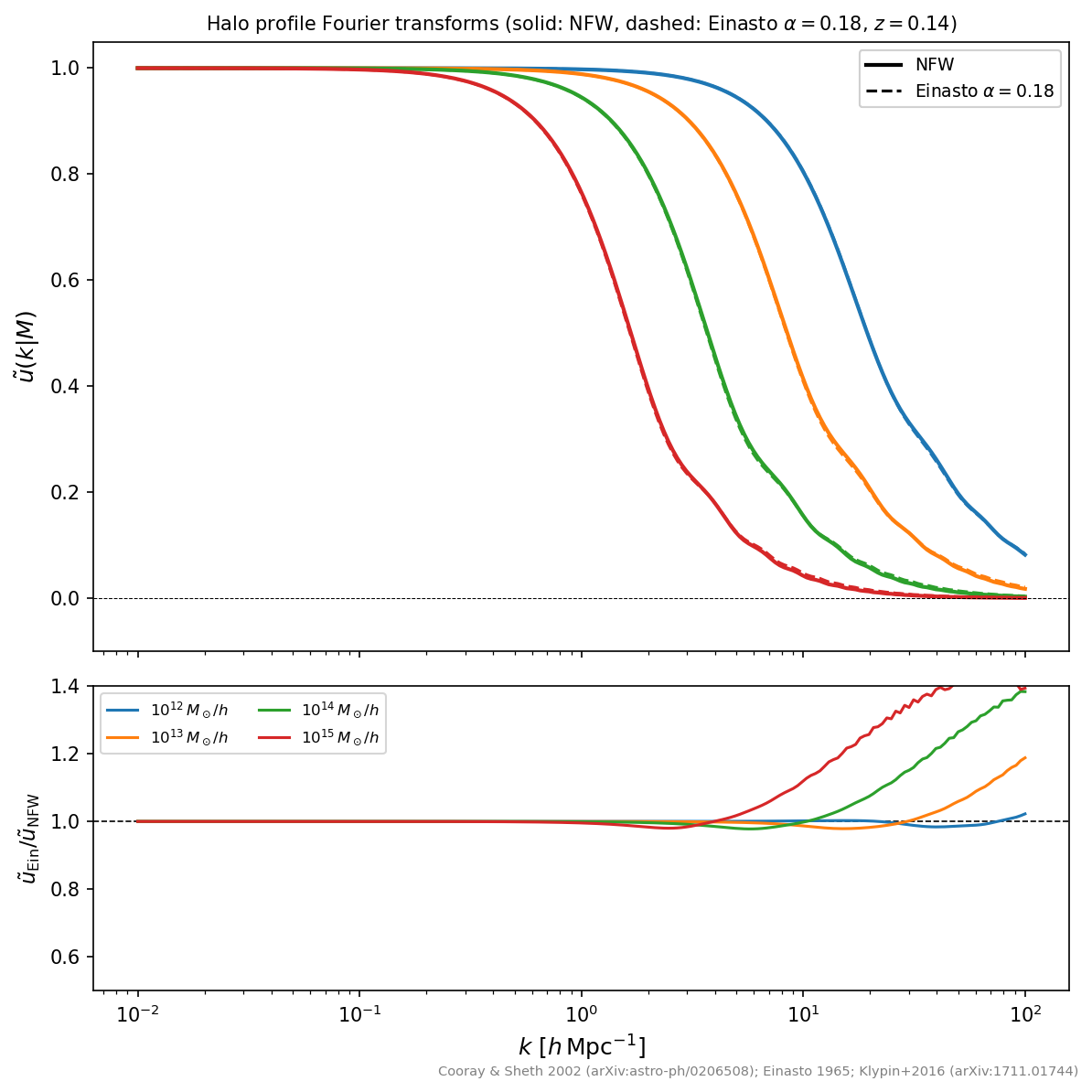
Normalised Fourier transforms \(\tilde{u}(k|M)\) of the NFW and Einasto profiles for several halo masses.
7. HOD Occupation Functions
The HOD specifies the mean number of central and satellite galaxies per halo
of mass \(M\). All nine models in hod_mod share the same interface:
N_cen, N_sat = hod.nc_ns(log10m_h, hod_params)
The galaxy number density and effective bias follow from:
Equations for each of the nine models follow.
Zheng+2007 (HODModel, arXiv:astro-ph/0703457):
Free params: log10mmin, σ_logm, log10m0, log10m1, α.
Kravtsov+2004 (Kravtsov04HODModel, ApJ 609, 35):
Same parameter names as HODModel; validated against the surhudm/aum code.
More+2015 (MoreHODModel, arXiv:1407.1856) — fiducial model for this showcase:
Incompleteness \(\alpha_{\rm inc} = \mathrm{clip}(1 + \alpha_{\rm inc,0} (\log_{10}M - \log_{10}M_{\rm inc}),\,0,\,1)\). For BGS, \(\alpha_{\rm inc}=1\).
Free params: log10mmin, σ_logm, log10m1, α, κ, α_inc, log10m_inc.
Zu & Mandelbaum 2015 iHOD (ZuMandelbaum15HODModel, arXiv:1505.02781):
The central SHMR maps halo mass to stellar mass via a 5-parameter model (ZM15 Eq. 19):
The central occupation for a stellar-mass threshold \(M_{*,{\rm thresh}}\):
with mass-dependent scatter \(\sigma_{\ln M_*}(M_h) = \sigma_{\ln M_*}(1 + \eta\log_{10}M_h)\). Satellites follow an exponential-cutoff power law.
Free params (with threshold): log10m_star_thresh, lg_m1h, lg_m0star, β, δ, γ, σ_lnM*, η, b_sat, α_sat (+2 more for M_cut, M_sat).
van Uitert+2016 CSMF (VanUitert16CSMFModel, arXiv:1601.06791):
Centrals selected in a stellar-mass bin \([M_{*,\rm lo},\,M_{*,\rm hi}]\) via a double power-law SHMR \(\mu(M_h)\):
Satellites follow a modified Schechter conditional stellar mass function \(\Phi_s(M_*|M_h)\) integrated over the stellar-mass bin.
Free params: log10m_h1, log10m_star0, β₁, log10_β₂, σ_c, α_s, b₀, b₁.
Zacharegkas+2025 (Zacharegkas25HODModel):
Uses the Kravtsov+2004 SHMR to invert a stellar-mass threshold into a halo-mass occupation function with Gaussian scatter in \(\log M_*\):
Satellites: \(\langle N_s \rangle = \langle N_c \rangle\,(M/M_{\rm sat})^{\beta_{\rm sat}}\).
Free params: log10m1_shmr, log10eps, α_shmr, γ_shmr, δ_shmr, σ_logm_star, α_sat, f_cen.
Guo+2018 ICSMF (Guo18ICSMFModel, arXiv:1804.01993):
Integrated conditional stellar mass function (ICSMF) — both centrals and satellites are derived from the CSMF \(\Phi(M_*|M_h)\), which combines a Gaussian central term and a Schechter satellite term. A mass-dependent incompleteness correction \(f_{\rm inc}(M)\) models survey selection.
Free params (14): 4 broken-PL SHMR + Gaussian width, 4 Schechter satellite + 2 incompleteness + 3 amplitude normalisation.
Guo+2019 ICSMF + quenching (Guo19ICSMFModel, arXiv:1810.05318):
Extends Guo+2018 with a quenched fraction for eBOSS ELGs: a critical mass \(\log_{10}M_q\) above which galaxies are quenched and therefore absent from the ELG selection.
Free params (15): all 14 from Guo+2018 + log10m_q.
Zu & Mandelbaum 2016/17 quenching (ZuMandelbaum16QuenchingModel,
arXiv:1509.06374):
Used on top of ZuMandelbaum15HODModel to split galaxies into red and blue.
The red fraction follows a Weibull (cumulative extreme-value) distribution:
Free params: lg_mqc_h, μ_c (centrals), lg_mqs_h, μ_s (satellites).
For BGS the incompleteness \(\alpha_{\rm inc}\) is fixed to 1 (the sample is >95% complete above the stellar mass threshold, arXiv:2512.15960).
Class |
Reference |
Free params |
Occupation type |
Key features / parametrisation |
|---|---|---|---|---|
|
Zheng+2007 (arXiv:astro-ph/0703457) |
5 |
Halo mass |
Baseline erfc \(N_c\), power-law \(N_s\); params: log10mmin, σ_logm, log10m0, log10m1, α |
|
More+2015 (arXiv:1407.1856) |
7 |
Halo mass |
Adds incompleteness α_inc and cut-off scale κ to Zheng+2007 |
|
Kravtsov+2004 (arXiv:astro-ph/0308519) |
5 |
Halo mass |
\(N_{\rm sat} = N_{\rm cen}(M/M_1)^\alpha \exp(-M_0/M)\);
same param names as |
|
Guo+2018 (arXiv:1804.01993) |
14 |
Stellar mass |
Broken power-law SHMR + mass-dependent completeness correction |
|
Guo+2019 (arXiv:1810.05318) |
15 |
Stellar mass |
Extends Guo+2018 with quenched fraction log10m_q for eBOSS ELGs |
|
Zu & Mandelbaum 2015 (arXiv:1505.02781) |
6 |
Stellar mass (iHOD) |
Inverse SHMR with log-normal scatter; \(N_c\) derived via JAX bisection inversion of the stellar-mass–halo-mass relation |
|
Zu & Mandelbaum 2016/17 |
— |
Stellar mass |
Weibull CDF red fractions for centrals and satellites; used on top
of |
|
van Uitert+2016 (arXiv:1601.06791) |
8 |
Stellar mass |
Gaussian conditional stellar mass function (CSMF) with flexible scatter and mass-dependent completeness |
|
Zacharegkas+2025 |
8 |
Stellar mass |
Kravtsov SHMR with threshold scatter; \(N_c\) via error function of the SHMR-inverted threshold |
References: More et al. 2015 (arXiv:1407.1856); Zheng et al. 2007 (arXiv:astro-ph/0703457); Zu & Mandelbaum 2015 (arXiv:1505.02781); van Uitert et al. 2016 (arXiv:1601.06791); Guo et al. 2018/19 (arXiv:1804.01993, arXiv:1810.05318).
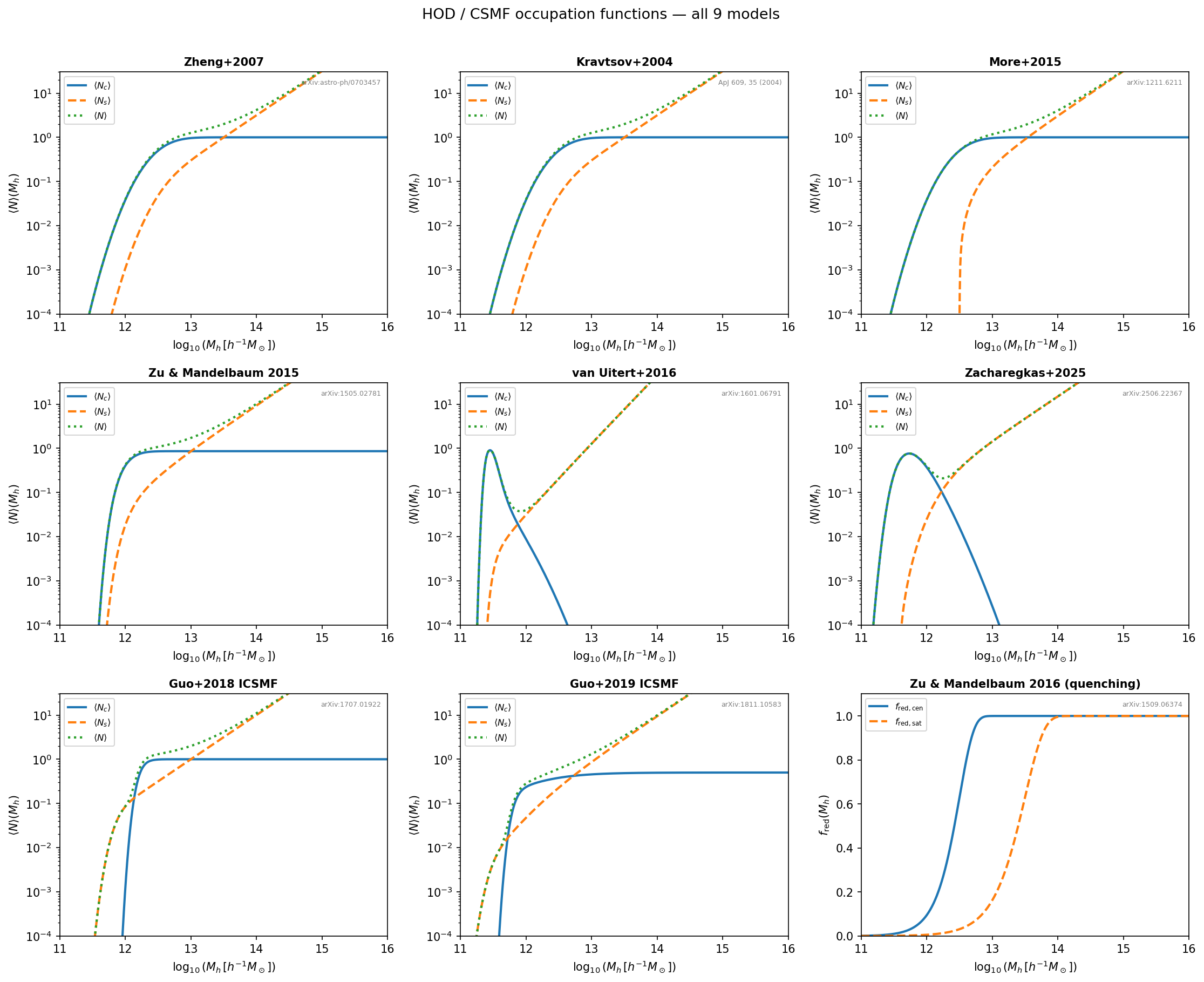
Mean central and satellite occupation functions \(\langle N_c\rangle(M)\) and \(\langle N_s\rangle(M)\) for all nine HOD models (3×3 panel).
HOD parameters in hod_mod are redshift-independent by default. The figure
below shows how the HOD-integrated observables \(\bar{n}_g\) and
\(b_{\rm eff}\) evolve purely because the HMF \({\rm d}n/{\rm d}M(M,z)\)
and halo bias \(b(M,z)\) change with redshift:
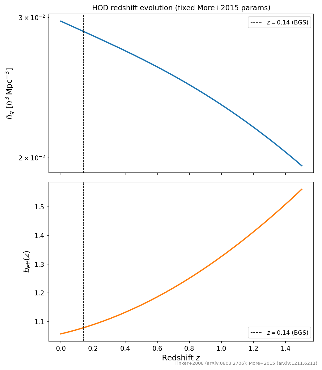
Galaxy number density \(\bar{n}_g(z)\) and effective bias \(b_{\rm eff}(z)\) for fixed HOD parameters, driven by HMF and \(b(M,z)\) evolution.
8. Off-centering Correction
Central galaxies are not always located at the potential minimum of their host halo. A fraction \(f_{\rm off}\) of centrals are displaced by a 2D projected offset drawn from a Rayleigh distribution with scale \(\sigma_{\rm off}\) [Mpc/\(h\)]. In Fourier space this averaging produces an isotropic damping factor for the central-galaxy contribution to the 1-halo power spectra (Johnston+2007 arXiv:0709.4193 Eq. A2; More+2015 arXiv:1407.1856 §3.3):
The effective central occupation entering both \(P_{gg}^{\rm 1h}\) and \(P_{gm}^{\rm 1h}\) becomes:
\(f_{\rm off} = 0\) (default): reduces exactly to the standard formula.
\(f_{\rm off} = 1\): all centrals are off-centered with scale \(\sigma_{\rm off}\).
At \(k \to 0\) (large scales): \(W_{\rm off} \to 1\) — the 2-halo regime is unaffected.
At \(k \gg 1/\sigma_{\rm off}\): the 1-halo contribution of centrals is exponentially suppressed, reducing \(\Delta\Sigma(R)\) and \(w_p(r_p)\) at \(R \lesssim \sigma_{\rm off}\).
Fits to BGS M★ > 10^10 at \(z_{\rm eff}=0.136\) recover \(f_{\rm off}\sim 0.13{-}0.15\), \(\sigma_{\rm off}\sim 0.2\) Mpc/\(h\), consistent with Leauthaud et al. 2012 (arXiv:1104.0928) group lensing results. The correction extends the usable WP scale from \(r_p > 0.3\) Mpc/\(h\) (without off-centering) to \(r_p > 0.1\) Mpc/\(h\) while maintaining \(\chi^2/{\rm dof} \lesssim 1.5\).
Enable with --use-offcentering; free parameters f_off ∈ [0, 1] and
sigma_off ∈ [0.01, 2.0] Mpc/\(h\) are added to the fit automatically.
References: Johnston et al. 2007 (arXiv:0709.4193); More et al. 2015 (arXiv:1407.1856) §3.3 + App. A; Leauthaud et al. 2012 (arXiv:1104.0928); Siegel et al. 2025 (arXiv:2209.07392).
9. Projected Correlation Function \(w_p(r_p)\)
The projected galaxy auto-correlation function integrates the 3D correlation function along the line of sight up to \(\pi_{\max}\):
The 3D correlation \(\xi_{gg}(r)\) is obtained from \(P_{gg}(k)\) via the Ogata (2005) Hankel transform. The power spectrum decomposes into:
where \(\Delta I_{\rm gg}^{\rm BNL}(k)\) is the beyond-linear bias correction
from BeyondLinearBiasMead21
(see section 4 for the full formula).
The BNL term boosts the 2-halo power at \(k \sim 0.05{-}0.8\,h\,{\rm Mpc}^{-1}\);
it vanishes at large scales (\(k < 6\times10^{-3}\,h\,{\rm Mpc}^{-1}\)).
The k-grid spans \([10^{-4}, 200]\,h/{\rm Mpc}\) (1024 points, log-spaced) to ensure accuracy of the Hankel transform down to \(r_p \approx 0.02\,h^{-1}{\rm Mpc}\).
References: More et al. 2015 (arXiv:1407.1856) Eqs. 9–10; Mead & Verde 2021 (arXiv:2011.08858) — BNL beyond-linear bias; Ogata 2005 Hankel transform.
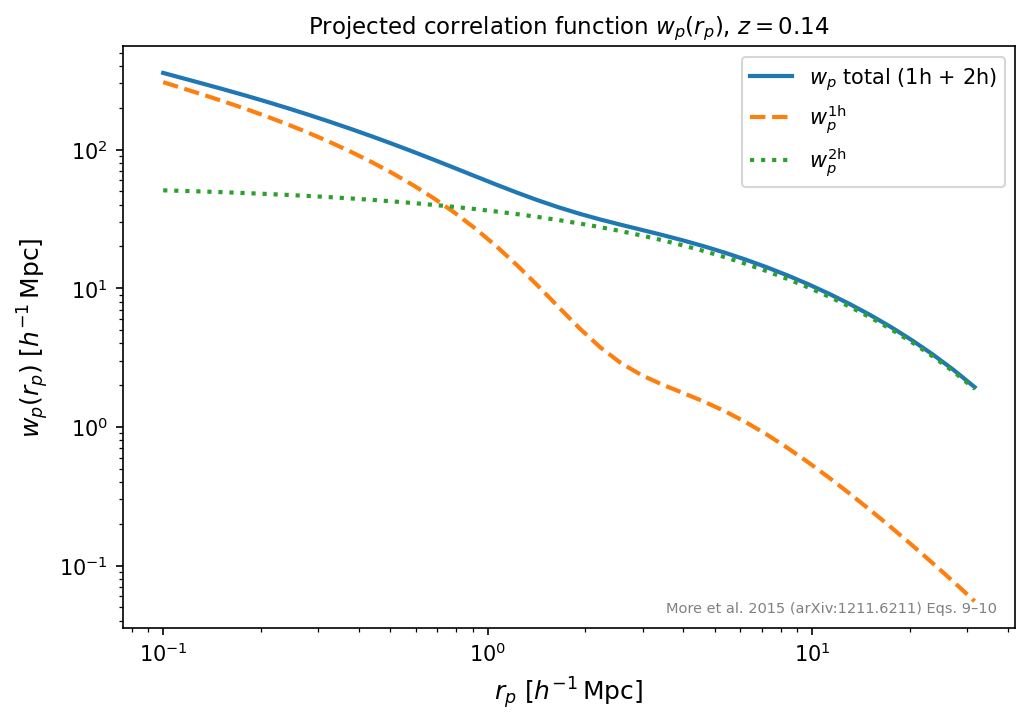
Projected correlation function \(w_p(r_p)\) with 1-halo and 2-halo decomposition for the fiducial More+2015 HOD.
10. Excess Surface Mass Density \(\Delta\Sigma(R)\)
The weak-lensing excess surface mass density is:
The galaxy–matter cross-correlation \(\xi_{gm}(r)\) is the Hankel transform of \(P_{gm}(k)\). The 1-halo term (More et al. 2015 arXiv:1407.1856 Eq. 13) reads:
where \(\Delta I_{\rm gm}^{\rm BNL}(k)\) is the asymmetric BNL correction defined in section 4.
The line-of-sight \(\chi\)-integral uses a log-linear hybrid grid (dense logarithmically at small \(\chi\), uniform at large \(\chi\)) for accurate convergence at both small and large \(R\).
References: More et al. 2015 (arXiv:1407.1856) Eq. 13; Mead & Verde 2021 (arXiv:2011.08858) — BNL beyond-linear bias; Bartelmann & Schneider 2001 (arXiv:astro-ph/9912508).
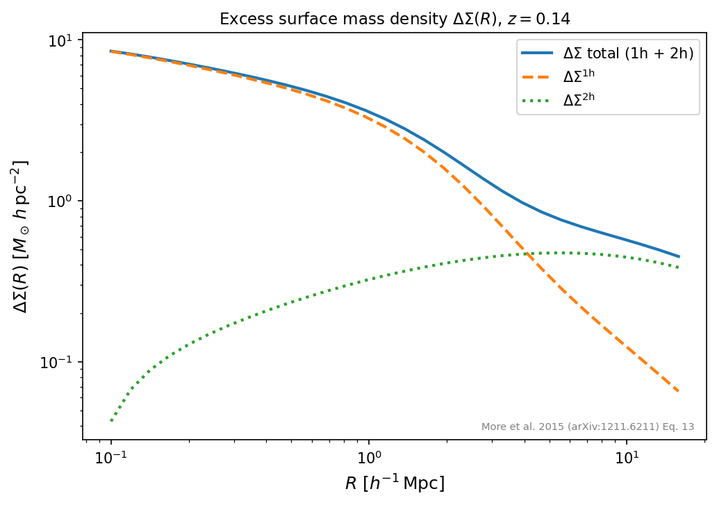
Excess surface mass density \(\Delta\Sigma(R)\) with 1-halo and 2-halo decomposition for the fiducial More+2015 HOD.
11. NLA Intrinsic-Alignment Correction to \(\Delta\Sigma\)
Lens galaxies are intrinsically aligned with the local tidal field, biasing the measured weak-lensing signal. The non-linear alignment (NLA) model (Bridle & King 2007 arXiv:0705.0166 §2) gives an additive correction:
with \(C_1\rho_{\rm crit,0} = 0.0134\) (Brown et al. 2002 arXiv:astro-ph/0208084) and \(D(z)\) the linear growth factor normalised to unity today.
Note
“Non-Linear Alignment” describes the physical mechanism (tidal alignment), not the use of a non-linear power spectrum. The input \(P_{\rm lin}\) is the physically correct choice (Bridle & King 2007 §2).
DESI KP6 finds \(A_{\rm IA} \sim 0.3{-}1.5\) for BGS-like lens samples (arXiv:2512.02954).
References: Bridle & King 2007 (arXiv:0705.0166); Brown et al. 2002 (arXiv:astro-ph/0208084); DESI KP6 (arXiv:2512.02954, arXiv:2509.04552).
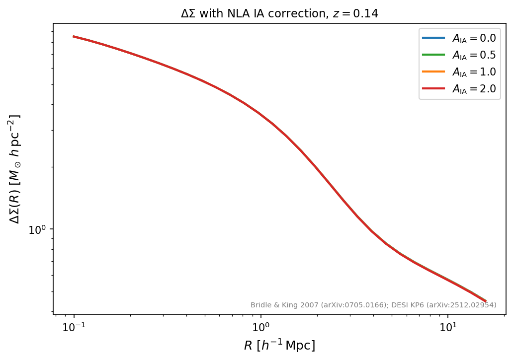
\(\Delta\Sigma(R)\) with the NLA intrinsic-alignment correction for \(A_{\rm IA} = 0,\,0.5,\,1,\,2\).
12. Summary: \(w_p\) — All Corrections
The figure below overlays the main physical effects on \(w_p(r_p)\):
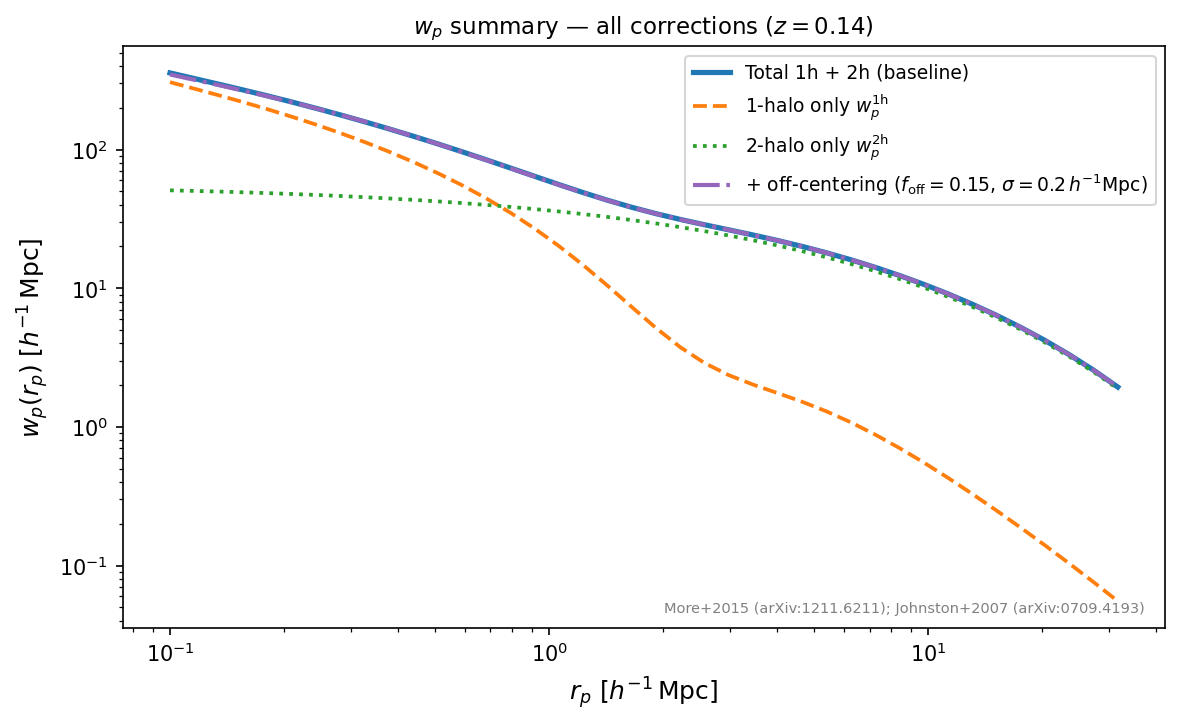
Summary of physical effects on \(w_p(r_p)\): total, 1-halo, 2-halo, and off-centering correction.
13. Summary: \(\Delta\Sigma\) — All Corrections
The figure below overlays the main physical effects on \(\Delta\Sigma(R)\):
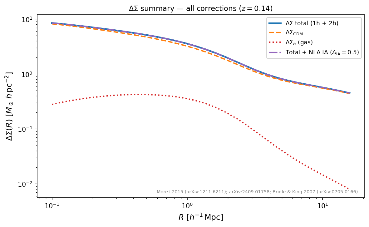
Summary of physical effects on \(\Delta\Sigma(R)\): total, 1-halo, 2-halo, and NLA intrinsic-alignment correction.
Galaxy × Gas Cross-Correlations
Beyond the standard \(w_p(r_p)\) and \(\Delta\Sigma(R)\) observables, hod_mod provides a complete halo model for cross-correlations between the galaxy overdensity field and diffuse gas signals:
Galaxy × tSZ Compton-y — \(P_{g,y}(k)\), the projected tSZ stack \(\Sigma_y(r_p)\), and the angular power spectrum \(C_\ell^{g,y}\). Uses the Arnaud et al. 2010 universal pressure profile.
Galaxy × soft X-ray (0.5–2 keV) — \(P_{g,X}(k)\) and the projected correlation \(w_{g,X}(r_p)\). Uses the DPM electron density profile of Oppenheimer et al. 2025.
Both signals are benchmarked against the eROSITA × Legacy Survey measurements of Comparat et al. 2025 (A&A 697, A173) for seven stellar-mass-selected galaxy samples (\(\log_{10}(M_*/M_\odot) > 10.0\), \(\ldots\), \(> 11.5\)).
Implementation classes
PressureProfileA10— A10 gNFW pressure profile; computes \(P_e(r|M,z)\) [keV/cm³] and \(\tilde{y}(k|M,z)\) [(Mpc/h)²].GasDensityDPM— DPM electron density profile; computes \(n_e(r|M,z)\) [cm⁻³], \(\tilde{n}_e(k|M,z)\) [(Mpc/h)³ cm⁻³], and \(\tilde\varepsilon(k|M,z)\) [(Mpc/h)³ cm⁻⁶].m200_to_m500c()— NFW bisection to convert M200m → M500c.HaloModelCrossSpectra— wraps an existingFullHaloModelPredictionand reuses its static cache to compute 1-halo + 2-halo cross-spectra and all projected observables.
Gas profile and cross-spectrum figures
Run the validation script to reproduce all seven diagnostic panels:
cd $HOD_MOD_REPO
python -m hod_mod.scripts.validate_sz_xray
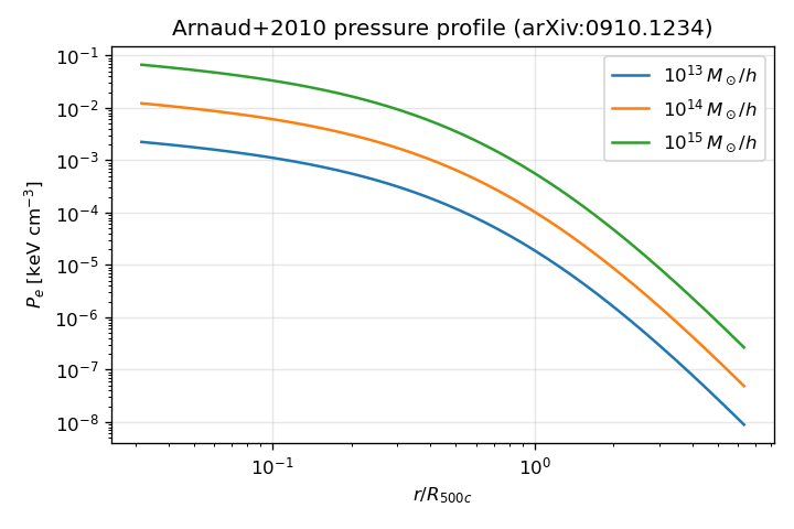
Figure SZ-1. Arnaud+2010 universal pressure profile \(P_e(r/R_{500c})\) [keV cm-3] for three halo masses (\(10^{13}\), \(10^{14}\), \(10^{15}\,M_\odot/h\)) at \(z=0.3\). Profile shape from arXiv:0910.1234, Eq. 11.
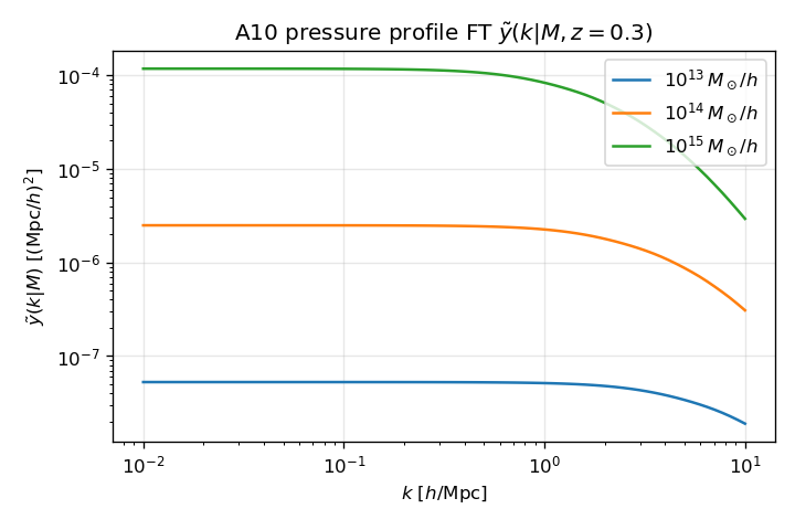
Figure SZ-2. Fourier transform \(\tilde{y}(k|M)\) [(Mpc/h)2] of the A10 pressure profile for the same three masses. The signal is flat at \(k \to 0\) and falls off at \(k \gtrsim 1/R_{500c}\).
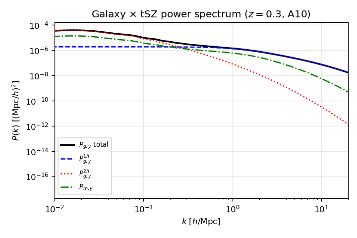
Figure SZ-3. Galaxy x tSZ cross-spectrum \(P_{g,y}(k)\) decomposed into 1-halo (dashed) and 2-halo (dotted) contributions, plus the total (solid) and the matter x tSZ term \(P_{m,y}(k)\). Computed with the More+2015 HOD and Planck 2018 cosmology at \(z=0.3\).
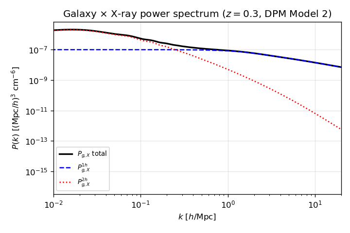
Figure SZ-4. Galaxy x soft X-ray cross-spectrum \(P_{g,X}(k)\) [(Mpc/h)3 cm-6] with 1-halo / 2-halo decomposition. Uses the DPM electron density profile (Model 2, arXiv:2505.14782) at \(z=0.3\).
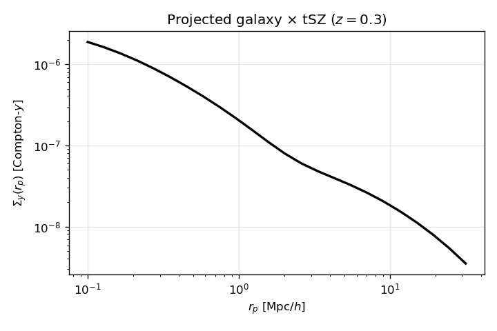
Figure SZ-5. Projected tSZ stacking signal \(\Sigma_y(r_p)\) [dimensionless Compton-y] vs projected radius \(r_p\) [Mpc/h]. Relevant for stacked ACT/SPT x BOSS measurements (cf. Amodeo+2021, arXiv:2009.05557).
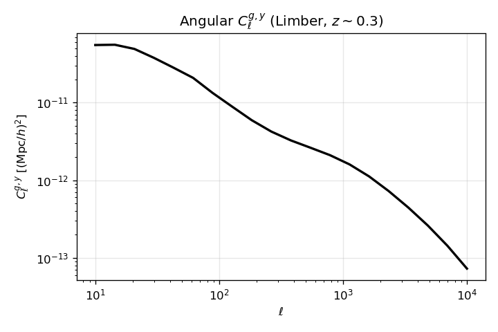
Figure SZ-6. Angular cross-power spectrum \(C_\ell^{g,y}\) via the Limber approximation for a BOSS CMASS-like \(n(z)\) at \(z_{\rm eff}=0.5\). Relevant for DES x ACT comparisons (cf. Pandey+2025, arXiv:2506.07432).
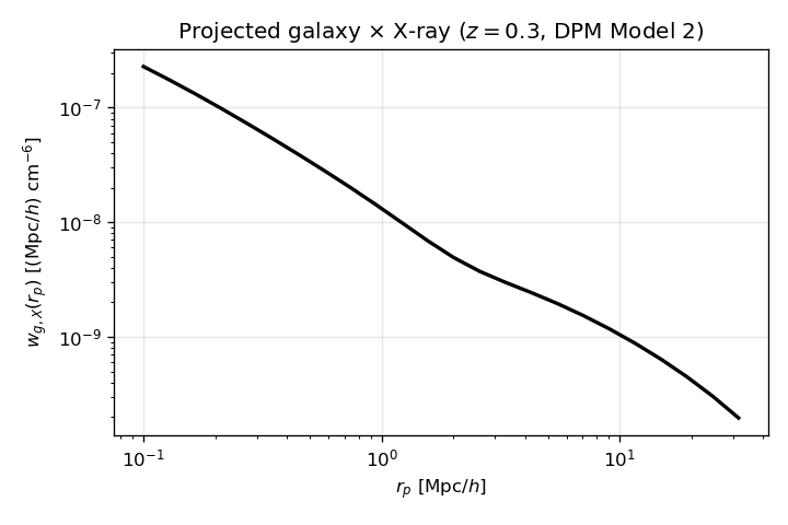
Figure SZ-7. Projected galaxy x soft X-ray correlation \(w_{g,X}(r_p)\) [(Mpc/h) cm-6] vs projected radius. Benchmarked against the eROSITA x Legacy Survey measurements of Comparat+2025 (arXiv:2503.19796, A&A 697, A173).
14. X-ray AGN Contribution to \(P_{g,X}(k)\)
AGN hosted in dark-matter halos contribute an X-ray surface brightness component to the galaxy × soft X-ray cross-correlation in addition to the diffuse thermal emission from the intra-group medium. Unlike thermal gas, AGN are unresolved point sources: their 3D density profile is a Dirac delta function, giving a flat Fourier transform \(\tilde{X}^{\rm AGN}(k|M) \propto \langle L_X(M,z)\rangle\).
The mean soft-band (0.5–2 keV) luminosity per halo is computed via
abundance-matching against the Aird+2015 LADE hard XLF
(see Galaxies Module § HAM AGN Model and HamAGNModel):
At each \((M_h, z)\) the cumulative AGN number density from the Aird+2015 LADE hard XLF is matched to the cumulative galaxy number density from the Girelli+2020 SHMR, giving \(\langle L_X^{\rm hard}(M_h, z)\rangle\).
Hard-to-soft conversion and obscuration are applied via a precomputed K-correction table integrating an absorbed power-law over \((z, \log N_H)\) (Comparat+2019 obscuration fractions).
The AGN component is added via the agn_model keyword of
HaloModelCrossSpectra:
from hod_mod.agn.ham import HamAGNModel
from hod_mod.observables.cross_spectra import HaloModelCrossSpectra

agn   = HamAGNModel(xlf="aird15")
cross = HaloModelCrossSpectra(fhmp, density_profile=dp, agn_model=agn)

# Retrieve gas and AGN contributions separately:
cl = cross.angular_cl_gX(ell, z_arr, nz_g, theta_cosmo, hod_params,
                          return_components=True)
cl_gas = cl["gas"]
cl_agn = cl["agn"]
At \(z_{\rm eff}=0.135\) with \(\log_{10}(M_*/M_\odot) > 10\):
The gas 1-halo term dominates at small angular scales (\(\ell \gtrsim 500\)).
The AGN 1-halo term is flat in \(\ell\) and becomes comparable at \(\ell \lesssim 100\).
The AGN 2-halo term (\(\propto b_{\rm eff}^2\,P_{\rm lin}\)) dominates at \(\ell \lesssim 50\).
Thread-safety note: angular_cl_gX calls CAMB at each redshift slice.
Always pass n_workers=1 to avoid non-deterministic NaN values in the
AGN 2-halo term when running from a multi-threaded context:
cl = cross.angular_cl_gX(..., n_workers=1)
References: Aird et al. 2015 (arXiv:1503.01120) — LADE hard XLF; Comparat et al. 2019 (arXiv:1901.10866) — HAM method and obscuration model; Girelli et al. 2020 (arXiv:2007.06220); Comparat et al. 2025 (arXiv:2503.19796).
Bibliography
See Bibliography for the full consolidated bibliography.
Key references for this showcase:
Planck 2018 (arXiv:1807.06209) — fiducial cosmology
Lewis, Challinor & Lasenby 2000 (arXiv:astro-ph/9911177) — CAMB
Aletheia 2025 (arXiv:2511.13826) — non-linear P(k) emulator
Brieden et al. 2025 WHM (arXiv:2508.10902) — Web-Halo Model non-linear P(k)
Tinker et al. 2008 (arXiv:0803.2706) — HMF
Tinker et al. 2010 (arXiv:1001.3162) — halo bias
Mead & Verde 2021 (arXiv:2011.08858) — beyond-linear halo bias \(\beta^{\rm NL}\) (BNL)
Navarro, Frenk & White 1997 (arXiv:astro-ph/9611107) — NFW profile
Diemer & Joyce 2019 (arXiv:1809.07326) — c–M relation
Cooray & Sheth 2002 (arXiv:astro-ph/0206508) — NFW Fourier transform
More et al. 2015 (arXiv:1407.1856) — HOD, P_gm, w_p, ΔΣ
Zheng et al. 2007 (arXiv:astro-ph/0703457) — HOD
Guo et al. 2018 (arXiv:1804.01993) — ICSMF HOD
Zu & Mandelbaum 2015 (arXiv:1505.02781) — iHOD
Bartelmann & Schneider 2001 (arXiv:astro-ph/9912508) — weak lensing
Bridle & King 2007 (arXiv:0705.0166) — NLA IA
Brown et al. 2002 (arXiv:astro-ph/0208084) — C1 normalisation
DESI KP6 (arXiv:2512.02954) — A_IA for BGS lenses
BGS HOD analysis (arXiv:2512.15960) — log10mmin priors
Einasto 1965 (Trudy Astrofiz. Inst. Alma-Ata 5, 87) — Einasto density profile
Klypin et al. 2016 (arXiv:1711.01744) — Einasto α=0.18 calibration
Johnston et al. 2007 (arXiv:0709.4193) — off-centering Fourier damping
Leauthaud et al. 2012 (arXiv:1104.0928) — group lensing f_off calibration
Zacharegkas et al. 2025 — Kravtsov SHMR HOD for DES galaxy groups
van Uitert et al. 2016 (arXiv:1601.06791) — CSMF HOD
Zu & Mandelbaum 2016 (arXiv:1509.06374) — Weibull quenching fractions
Mead et al. 2020 HMcode-2020 (arXiv:2009.01858) — CAMB non-linear P(k)
Takahashi et al. 2012 (arXiv:1208.2701) — CAMB HALOFIT revised
Duffy et al. 2008 (arXiv:0804.2486) — NFW concentration–mass relation
Dutton & Macciò 2014 (arXiv:1402.7073) — concentration–mass relation
Prada et al. 2012 (arXiv:1104.5130) — concentration–mass relation
Press & Schechter 1974 (ApJ 187, 425) — original HMF
Sheth & Tormen 1999 (arXiv:astro-ph/9901122) — ellipsoidal collapse HMF
Warren et al. 2006 (arXiv:astro-ph/0506395) — N-body-calibrated HMF
Watson et al. 2013 (arXiv:1212.0095) — FoF HMF
Bocquet et al. 2016 (arXiv:1502.07357) — DM-only HMF
Arnaud et al. 2010 (arXiv:0910.1234) — A10 universal pressure profile
Oppenheimer et al. 2025 (arXiv:2505.14782) — DPM electron density profile
Comparat et al. 2025, A&A 697, A173 (arXiv:2503.19796) — galaxy × eROSITA benchmark
Amodeo et al. 2021 (arXiv:2009.05557) — ACT × BOSS CMASS/LOWZ stacked tSZ
Pandey et al. 2025 (arXiv:2506.07432) — DES × ACT DR6 lensing × tSZ
Comparat et al. 2019 (arXiv:1901.10866) — AGN X-ray luminosity–stellar mass abundance matching framework
Hasinger, Miyaji & Schmidt 2005 (arXiv:astro-ph/0506118) — LDDE soft XLF used to calibrate \(a\), \(b\), and the duty cycle evolution
Girelli et al. 2020 (arXiv:2007.06220) — stellar-to-halo mass relation (SHMR) used by
XrayAGNModel