Zu & Mandelbaum 2015 iHOD Model — SDSS, X-ray & BGS
Model class |
|
Paper |
Zu & Mandelbaum 2015, MNRAS 454, 1161 (arXiv:1505.02781) |
SHMR basis |
Behroozi, Converse & Wechsler 2010, ApJ 717, 379 (arXiv:1001.0015) |
Survey (benchmark) |
SDSS DR7, \(\log_{10}(M_*/h^{-2}M_\odot) > 10.2\), \(z_\mathrm{eff} \approx 0.1\) |
Observable (benchmark) |
Joint \(w_p(r_p) + \Delta\Sigma(R)\), \(\pi_\mathrm{max} = 60\,h^{-1}\,\mathrm{Mpc}\), 11 bins each (\(r_p,\,R \in [0.05,\,20]\,h^{-1}\,\mathrm{Mpc}\)) |
X-ray extension |
BGS LS10 × eROSITA (0.5–2 keV), Comparat et al. 2025 (arXiv:2503.19796) |
Code |
|
Cosmological framework
Both HOD models share the same backbone; see also More+2015 HOD Model — BOSS CMASS & BGS.
Cosmological parameters
Six base parameters \(\boldsymbol{\theta} = (\Omega_m,\,\Omega_b,\,h,\,n_s,\,\ln 10^{10}A_s,\,\sigma_8)\)
define the linear matter power spectrum \(P_\mathrm{lin}(k, z)\) via
CAMB (LinearPowerSpectrum).
Benchmark cosmology (ZM15-specific): \(\Omega_m = 0.260,\ h = 0.720,\ \sigma_8 = 0.770,\ n_s = 0.960,\ \Omega_b = 0.044\).
BGS/LS10 X-ray fits use Planck 2018: \(\Omega_m = 0.315,\ h = 0.674,\ \sigma_8 = 0.811,\ n_s = 0.965\).
Halo mass function
Tinker et al. 2008 (arXiv:0803.2706),
\(\Delta = 200\rho_m\), via
make_hmf()
with backend="tinker08" (default).
Alternative emulator backends — "csst" (Chen+2025,
SCPMA 2025)
and "aemulusnu" (Shen+2025,
arXiv:2410.00913) — expose the
same interface; see Cosmology Module for details.
Note
The BGS×eROSITA fit (hod_mod.scripts.fitting.fit_comparat2025) uses
the CSST emulator HMF by default, and the same HMF instance is reused by
the AGN model (HamAGNModel accepts an hmf= argument)
so the galaxy clustering and the AGN model share one consistent
mass function rather than each defaulting to Tinker08.
Linear halo bias
Tinker et al. 2010 (arXiv:1001.3162), with
the beyond-linear halo bias correction of Mead & Verde 2021
(arXiv:2011.08858;
BeyondLinearBiasMead21) applied
to the 2-halo galaxy terms. The BGS×eROSITA fit passes this bnl_model into
FullHaloModelPrediction so the non-linear
scale-dependent bias is used consistently in \(w_p\) and \(w_\theta\).
Effective bias:
NFW profile and Fourier transform
NFW profile (Navarro, Frenk & White 1997, arXiv:astro-ph/9508025); Fourier transform from Cooray & Sheth 2002 (arXiv:astro-ph/0206508), concentration–mass from Diemer & Joyce 2019 (arXiv:1809.07326).
Zu & Mandelbaum 2015 iHOD model
Unlike traditional HOD models that parametrise \(N(M_h)\) directly, the
inverse HOD (iHOD) derives the halo occupation from the stellar-to-halo
mass relation (SHMR) by inversion: the mean stellar mass
\(M_*^\mathrm{c}(M_h)\) is obtained by inverting the SHMR, and the
occupation functions follow from the log-normal scatter around that mean.
This is equivalent to the conventional HOD (cHOD) at the 1–2% level for
\(w_p\) and \(\Delta\Sigma\) (verified in
results/benchmarks/zumandelbaum2015_sdss/comparison_ihod_chod_wp_ds.png).
Implementation: ZuMandelbaum15HODModel
whose nc_ns() method
returns \((N_c,\,N_s)\) arrays consumed by
FullHaloModelPrediction.
Pedagogical figures and tutorial notebook
Each equation below is illustrated by a figure produced by
hod_mod/scripts/benchmarks/illustrate_zumandelbaum2015_equations.py
(run it to regenerate the panels, or pass --to-notebook to export the
interactive tutorial notebooks/zumandelbaum2015_equations.ipynb). The
occupation equations (Eqs. 19–22) are cosmology-independent and additionally
show their analytic jax.grad parameter sensitivity; the clustering
observables (\(b_\mathrm{eff}\), \(P(k)\), \(w_p\),
\(\Delta\Sigma\)) carry a bottom panel with the logarithmic
sensitivity \(d\ln O/d\ln p\) to \(\Omega_m\), \(\sigma_8\)
and \(h\) (central finite differences, since CAMB lies outside the JAX
graph), with the top panel overlaying \(+2\%\) variants.
Step 1 — SHMR forward direction (ZM15 Eq. 19)
The SHMR is written as halo mass as a function of stellar mass (Behroozi et al. 2010, ZM15 Eq. 19):
where \(M_1 = 10^{\mathtt{lg\_m1h}}\) and
\(M_{*,0} = 10^{\mathtt{lg\_m0star}}\) are the pivot halo and stellar
masses.
Implemented in _mh_from_mstar_zu15().
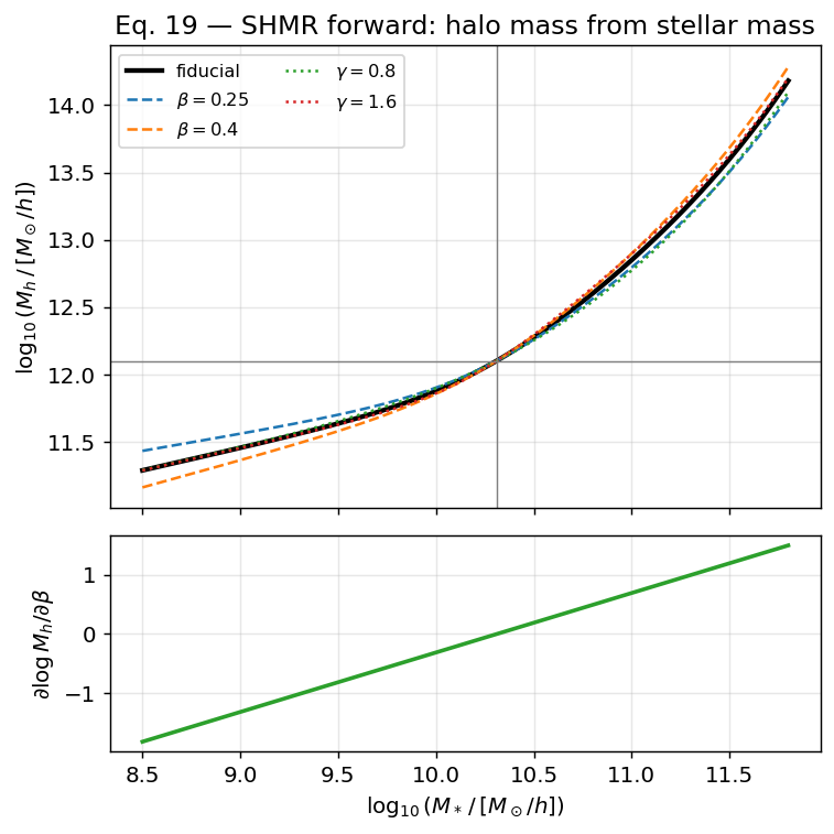
SHMR forward direction (Eq. 19). Sweeping the low-mass slope
\(\beta\) and transition sharpness \(\gamma\) pivots the relation
about \((M_{*,0}, M_1)\). Lower panel: the analytic
\(\partial\log_{10}M_h/\partial\beta\) from jax.grad.
Step 2 — SHMR inversion: mean stellar mass at fixed \(M_h\)
The iHOD requires \(M_*(M_h)\) — the mean stellar mass of a central galaxy in a halo of mass \(M_h\). Because Eq. 19 has no closed-form inverse, it is numerically inverted by 60 iterations of JAX-compatible bisection over \(\log_{10}(M_*/M_\odot) \in [4, 13]\):
implemented in _mstar_from_mh_zu15().
The 60-iteration bisection converges to \(\lesssim 10^{-17}\) dex
precision; in practice the output is accurate to machine precision for any
\(M_h \in [10^{10},\,10^{15.5}]\,M_\odot/h\).
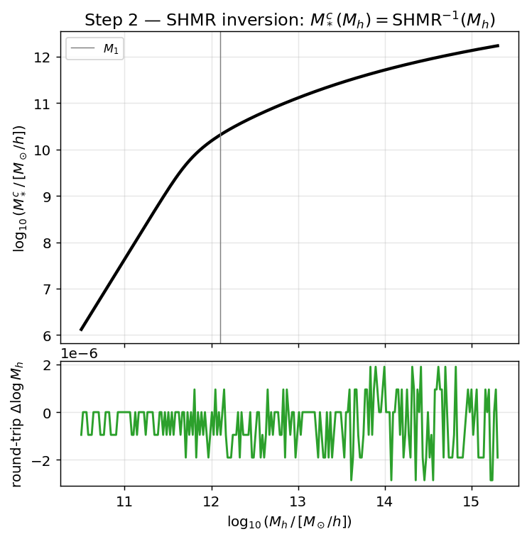
SHMR inversion. The mean central stellar mass \(M_*^\mathrm{c}(M_h)\) from the JAX bisection. Lower panel: the forward-of-inverse round-trip residual sits at the \(\sim10^{-14}\) dex floor, confirming machine-precision inversion.
Step 3 — Mass-dependent scatter in \(\ln M_*\) (ZM15 Eq. 20)
The log-normal scatter in stellar mass at fixed halo mass varies with \(M_h\):
\(\eta < 0\) encodes decreasing scatter toward cluster-scale halos
(ZM15 best fit \(\eta = -0.04\)).
Implemented in sigma_lnmstar_zu15().
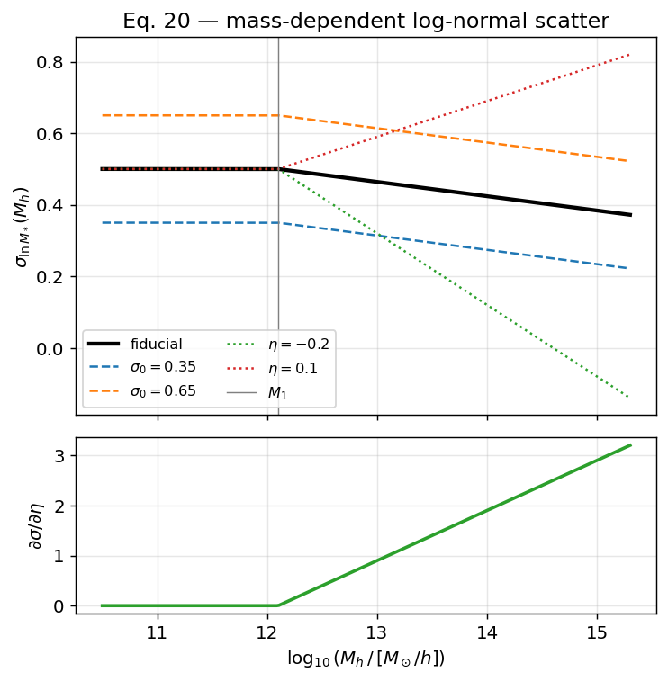
Mass-dependent scatter (Eq. 20). The scatter is flat below the pivot
\(M_1\) and tilts with slope \(\eta\) above it. Lower panel:
\(\partial\sigma/\partial\eta\) from jax.grad switches on exactly at
\(M_1\).
Step 4 — Central occupation (ZM15 Eq. 21)
\(M_{*,\mathrm{th}}\) is the stellar-mass threshold that defines
the galaxy sample: only galaxies with stellar mass
\(M_* \geq M_{*,\mathrm{th}}\) are counted.
It is set by the parameter log10m_star_thresh
(\(= \log_{10}(M_{*,\mathrm{th}}/M_\odot)\)).
Key iHOD step. Assuming \(\ln M_*\,|\,M_h\) is Gaussian with mean \(\ln M_*^\mathrm{c}(M_h)\) and standard deviation \(\sigma_{\ln M_*}(M_h)\), the probability that the central galaxy satisfies \(M_* > M_{*,\mathrm{th}}\) is:
\(f_c \leq 1\) is a central-galaxy completeness fraction
(see note below). At the characteristic halo mass
\(M_h = M_\mathrm{min} \equiv \mathrm{SHMR}^{-1}(M_{*,\mathrm{th}})\),
the argument of erfc vanishes and
\(\langle N_\mathrm{cen}\rangle = f_c/2\).
Implemented in n_cen_thresh_zu15().
Note
In the original ZM15 paper, \(f_c\) is defined as the satellite concentration ratio (\(c_\mathrm{sat} = f_c\,c_\mathrm{dm}\), Table 2, Section 4.4) and does not appear in \(\langle N_\mathrm{cen}\rangle\). This implementation repurposes \(f_c\) as a central-galaxy completeness fraction — an extension useful for flux-limited samples. The ZM15 best-fit value (0.86) is adopted as the default.
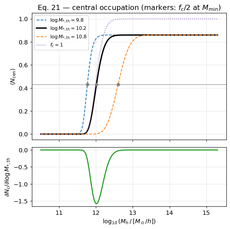
Central occupation (Eq. 21). Raising the threshold
\(M_{*,\mathrm{th}}\) shifts the erfc step to higher halo mass; the grey
markers sit at \(f_c/2\) at \(M_\mathrm{min}\). Lower panel: the
jax.grad threshold sensitivity peaks at the transition mass.
Step 5 — Satellite mass scales (ZM15 Eq. 22 auxiliary)
The characteristic halo mass \(M_\mathrm{min}\) for the threshold sample is obtained directly from the SHMR (no iteration needed here — the forward direction Eq. 19 is used):
Then the satellite mass scale and cut-off mass follow:
computed inside n_sat_thresh_zu15() before the
power-law occuption is evaluated.
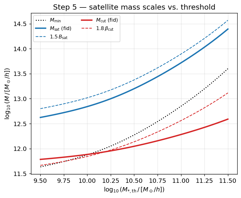
Satellite mass scales (Step 5). \(M_\mathrm{sat}\) (per-satellite mass) and \(M_\mathrm{cut}\) (truncation mass) as functions of the threshold, tied to \(M_\mathrm{min}\) through the SHMR; dashed curves vary \(B_\mathrm{sat}\) and \(\beta_\mathrm{cut}\).
Step 6 — Satellite occupation (ZM15 Eq. 22)
The satellite occupation inherits \(\langle N_\mathrm{cen}\rangle\) as
a prefactor, so it vanishes for halos that are too light to host a central
galaxy above the threshold.
Implemented in n_sat_thresh_zu15().
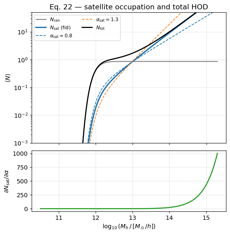
Satellite and total occupation (Eq. 22). Satellites inherit the central
prefactor (vanishing in light halos), rise as a power law of slope
\(\alpha_\mathrm{sat}\), and are cut below \(M_\mathrm{cut}\). Lower
panel: the jax.grad \(\alpha_\mathrm{sat}\) sensitivity grows toward
massive halos.
Step 7 — Stellar-mass bin HOD (used in joint fit)
When fitting stellar-mass bins rather than threshold samples (as in
hod_mod.scripts.fitting.bgs_ls10.fit_bgs_zm15_joint), the bin HOD
is computed by subtraction of two threshold HODs at the bin edges
\([M_{*,\mathrm{lo}},\,M_{*,\mathrm{hi}})\):
This is activated by passing log10m_star_max in hod_params to
nc_ns().
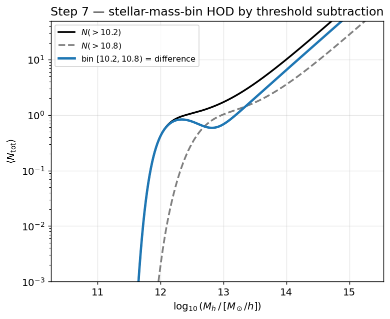
Stellar-mass-bin HOD (Step 7). The occupation of a stellar-mass bin is the difference of the two threshold HODs at the bin edges.
Step 8 — Standard halo-model integrals
Once \((N_c(M_h),\,N_s(M_h))\) are in hand, all clustering
predictions follow the standard halo-model framework — shared with the
More+2015 path in FullHaloModelPrediction:
The difference from a pure cHOD model is that \(N_c(M_h)\) and \(N_s(M_h)\) are derived from the SHMR inversion (Steps 1–4) rather than fitted directly in halo-mass space. For the BGS samples analysed here, the iHOD and cHOD predictions agree to ≲1–2% (see comparison figure in the SDSS benchmark section below).
wp(),
delta_sigma(),
and n_gal()
all follow this path.
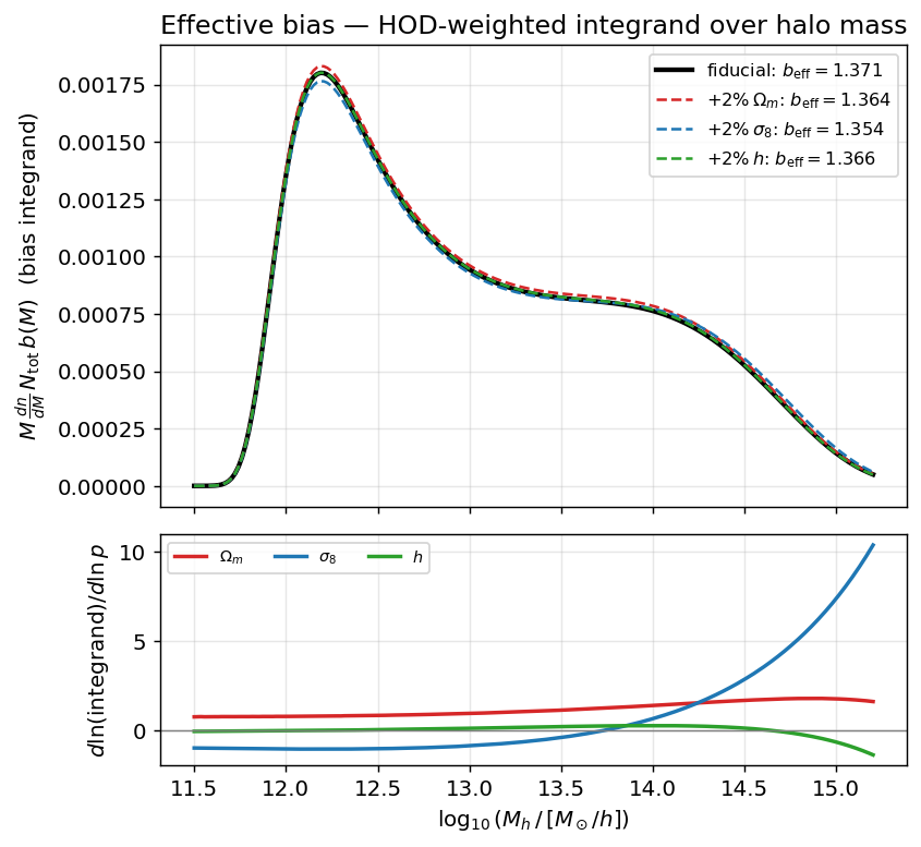
Effective bias — the first cosmology-dependent quantity. The HOD-weighted bias integrand \(M\,\frac{dn}{dM}\,N_\mathrm{tot}\,b(M)\) for the fiducial cosmology and three \(+2\%\) variants, with \(b_\mathrm{eff}\) quoted in the legend. Lower panel: the logarithmic sensitivity \(d\ln(\mathrm{integrand})/d\ln p\) to \(\Omega_m\), \(\sigma_8\) and \(h\) (central finite differences).
Power spectra and summary statistics
The power spectra and projected statistics follow the same formalism as More+2015 HOD Model — BOSS CMASS & BGS.
1-halo power spectra (galaxy auto + galaxy–matter):
2-halo power spectra:
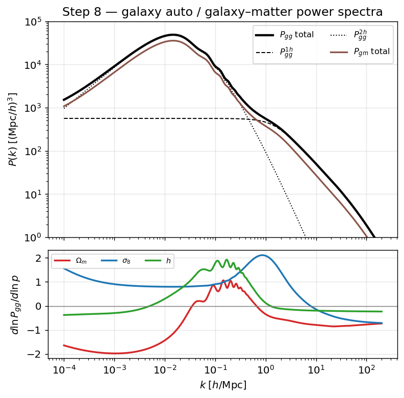
Galaxy auto / galaxy–matter power spectra. The 1-halo term dominates at high \(k\), the 2-halo term at low \(k\). Lower panel: the logarithmic sensitivity \(d\ln P_{gg}/d\ln p\) to \(\Omega_m\), \(\sigma_8\) and \(h\). The \(\sigma_8\) curve is nearly flat at \(\simeq2\) (\(P\propto\sigma_8^2\)), while \(\Omega_m\) and \(h\) are scale-dependent (central finite differences).
Projected correlation function (\(\pi_\mathrm{max} = 60\,h^{-1}\,\mathrm{Mpc}\) for SDSS):
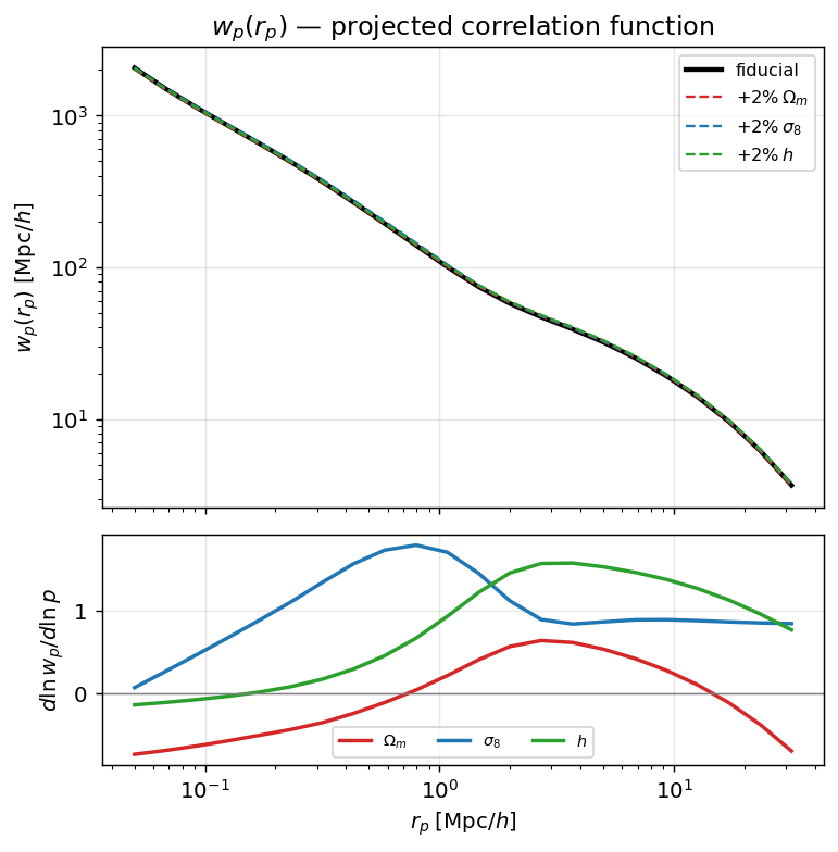
Projected correlation function \(w_p(r_p)\). Top panel overlays the fiducial with three \(+2\%\) variants. Lower panel: the logarithmic sensitivity \(d\ln w_p/d\ln p\) to \(\Omega_m\), \(\sigma_8\) and \(h\), each with a distinct scale dependence (central finite differences).
Excess surface density:
\(\xi(r)\) is computed via the Ogata (2005) \(j_0\) Hankel transform (DOI:10.2977/prims/1145474602).
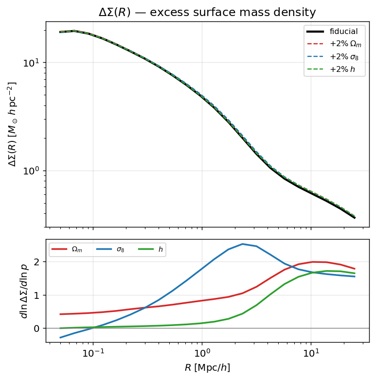
Excess surface mass density \(\Delta\Sigma(R)\). Because \(\Sigma_{gm}\propto\bar\rho_m\propto\Omega_m\), the signal is especially sensitive to \(\Omega_m\) — visible in the lower panel, the logarithmic sensitivity \(d\ln\Delta\Sigma/d\ln p\) to \(\Omega_m\), \(\sigma_8\) and \(h\) (central finite differences).
Predicting the stellar mass function \(\Phi(M_*)\)
Because the iHOD occupation functions are defined as a function of a stellar-mass threshold \(M_{*,\mathrm{th}}\) rather than a stellar-mass bin, the model does not return \(\Phi(M_*)\) directly. It is obtained by first computing the cumulative galaxy number density above a threshold, then differentiating numerically.
Step 1 — cumulative number density. For a fixed set of iHOD parameters \((\log_{10}M_1,\,\log_{10}M_{*,0},\,\beta,\,\delta,\,\gamma,\, \sigma_{\ln M_*},\,\eta,\,f_c,\,B_\mathrm{sat},\,\beta_\mathrm{sat},\, B_\mathrm{cut},\,\beta_\mathrm{cut},\,\alpha_\mathrm{sat})\), the central and satellite occupation functions above threshold (\(\langle N_\mathrm{cen}(M_h\,|\,M_{*,\mathrm{th}})\rangle\), \(\langle N_\mathrm{sat}(M_h\,|\,M_{*,\mathrm{th}})\rangle\) from Eqs. 21–22 above) are integrated against the halo mass function:
implemented in
n_gal()
(its hod_params["log10m_star_thresh"] entry is
\(\log_{10}M_{*,\mathrm{th}}\), in \(\log_{10}(M_\odot\,h^{-1})\)
— see the parameter table below).
Step 2 — finite-difference derivative. Evaluating \(\bar n_g(>M_{*,\mathrm{th}})\) on a grid of thresholds and differentiating gives the differential stellar mass function:
i.e. \(\Phi(M_*)\,\mathrm{d}\log_{10}M_*\) is the number density of
galaxies with stellar mass in \([M_*,\,M_* + \mathrm{d}M_*]\). This is
implemented by a centred finite difference
(numpy.gradient()) over the threshold scan — no closed-form derivative
of Eqs. 21–22 is taken, so the same code path works for any iHOD
parameter set without re-deriving the SHMR algebra.
Units (h convention). The sum_stat SMF data \(\Phi\) is tabulated in
\(h^3\,\mathrm{Mpc}^{-3}\,\mathrm{dex}^{-1}\) (= \((\mathrm{Mpc}/h)^{-3}\,\mathrm{dex}^{-1}\);
see smf()), the same
numeric convention as the halo model’s native comoving density
\(\mathrm{d}n/\mathrm{d}M\;[(\mathrm{Mpc}/h)^{-3}/(M_\odot/h)]\). The model
\(\bar n_g\) is therefore returned directly in \((\mathrm{Mpc}/h)^{-3}\)
with no \(h^3\) factor (the mass axis is still converted to the SHMR
convention by the \(+\log_{10}h\) threshold shift). An earlier version
multiplied by \(h^3\), under-predicting the SMF by \(h^3\approx0.31\)
(_predict_smf()).
SMF entry in the likelihood — number density only
The binned \(\Phi(M_*)\) is not fit shape-by-shape. Two issues make that pathological for the LS10-BGS samples: (i) the joint SMF+wp jackknife covariance is numerically near-singular (condition number \(\sim10^{16}\), SMF variances \(\sim10^{-13}\) vs \(w_p\) \(\sim10^{2}\)), so its dense inverse is meaningless; and (ii) the iHOD over-predicts the high-mass SMF tail (\(\gtrsim 3\text{--}30\times\) at \(\log_{10}M_*\gtrsim11.5\), where the small \(z<0.18\) volume is also unreliable), which — with tiny per-bin errors — railed \(f_c\) and the threshold against their bounds.
Instead the joint galaxy-sector likelihood uses diagonal uncertainties on \(w_p(r_p)\) plus a single overall number-density constraint,
compared to \(\int \Phi\,\mathrm{d}\log_{10}M_*\) from the data with a systematic floor (\(f_\mathrm{sys}\), default 5%). This is robust to the high-mass shape mismatch while still pinning the overall galaxy abundance. \(\Phi(M_*)\) itself (h³-correct) is retained for the diagnostic panels.
Parameter table
Parameter |
Symbol |
Default |
Fitted? |
ZM15 Table 2 (\(\pm 1\sigma\)) |
Units |
|---|---|---|---|---|---|
|
\(\log_{10} M_{*,\mathrm{th}}\) |
10.2 |
Yes |
— (sample-specific) |
\(\log_{10}(M_\odot h^{-2})\) |
|
\(\log_{10} M_1\) |
12.10 |
Yes |
\(12.10 \pm 0.17\) |
\(\log_{10}(M_\odot h^{-1})\) |
|
\(\log_{10} M_{*,0}\) |
10.31 |
Yes |
\(10.31 \pm 0.10\) |
\(\log_{10}(M_\odot h^{-2})\) |
|
\(\beta\) |
0.33 |
Yes |
\(0.33 \pm 0.21\) |
— |
|
\(\delta\) |
0.42 |
Yes |
\(0.42 \pm 0.04\) |
— |
|
\(\gamma\) |
1.21 |
Yes |
\(1.21 \pm 0.20\) |
— |
|
\(\sigma_{\ln M_*}\) |
0.50 |
Yes |
\(0.50 \pm 0.04\) |
— |
|
\(\eta\) |
−0.04 |
Yes |
\(-0.04 \pm 0.02\) |
— |
|
\(f_c\) |
0.86 |
Yes |
\(0.86 \pm 0.14\) |
— |
|
\(B_\mathrm{sat}\) |
8.98 |
Yes |
\(8.98 \pm 1.18\) |
— |
|
\(\beta_\mathrm{sat}\) |
0.90 |
Fixed |
— |
— |
|
\(B_\mathrm{cut}\) |
0.86 |
Fixed |
— |
— |
|
\(\beta_\mathrm{cut}\) |
0.41 |
Fixed |
— |
— |
|
\(\alpha_\mathrm{sat}\) |
1.00 |
Fixed (SDSS); Yes (BGS) |
— |
— |
SDSS DR7 benchmark
Source: results/benchmarks/zumandelbaum2015_sdss/benchmark_result.json.
Data digitised from ZM15 Figure 6 (WebPlotDigitizer);
reference data also from Mandelbaum et al. 2006
(arXiv:astro-ph/0509702).
Warning
This is not a parameter-recovery validation.
The v0.3 re-run gives \(\chi^2/\mathrm{dof} = 0.8095/13 =
0.0623\) — a good fit, but the parameters it fits with are not
the published ones. delta and gamma sit exactly on their prior
ceilings (2.0 and 5.0), i.e. \(+39.5\sigma\) and \(+19.0\sigma\)
from ZM15, and eta is \(+5.9\sigma\) off. A near-zero
\(\chi^2\) reached with two parameters railed against a bound is a
degenerate solution, not agreement.
The MCMC says the same thing more plainly: the marginal posteriors span
essentially the whole prior box (lg_m1h 11.0–14.0, delta 0.1–2.0,
gamma 0.5–5.0), so these 13 digitised \(w_p\) + \(\Delta\Sigma\)
points do not constrain the nine iHOD parameters. The earlier text here
claimed \(\chi^2/\mathrm{dof} \approx 1.75\times10^{-6}\) and
“\(0.00\sigma\) across the board”; that was measured before the 0.3.0
Hankel-transform fix and is superseded.
Parameter |
MAP |
Published (\(\pm 1\sigma\)) |
Deviation |
|---|---|---|---|
|
12.2202 |
\(12.10 \pm 0.17\) |
\(+0.71\sigma\) |
|
10.2426 |
\(10.31 \pm 0.10\) |
\(-0.67\sigma\) |
|
0.2642 |
\(0.33 \pm 0.21\) |
\(-0.31\sigma\) |
|
2.0000 ⚠ at prior bound |
\(0.42 \pm 0.04\) |
\(+39.50\sigma\) |
|
5.0000 ⚠ at prior bound |
\(1.21 \pm 0.20\) |
\(+18.95\sigma\) |
|
0.6266 |
\(0.50 \pm 0.04\) |
\(+3.16\sigma\) |
|
0.0770 |
\(-0.04 \pm 0.02\) |
\(+5.85\sigma\) |
|
0.5528 |
\(0.86 \pm 0.14\) |
\(-2.19\sigma\) |
|
8.7904 |
\(8.98 \pm 1.18\) |
\(-0.16\sigma\) |
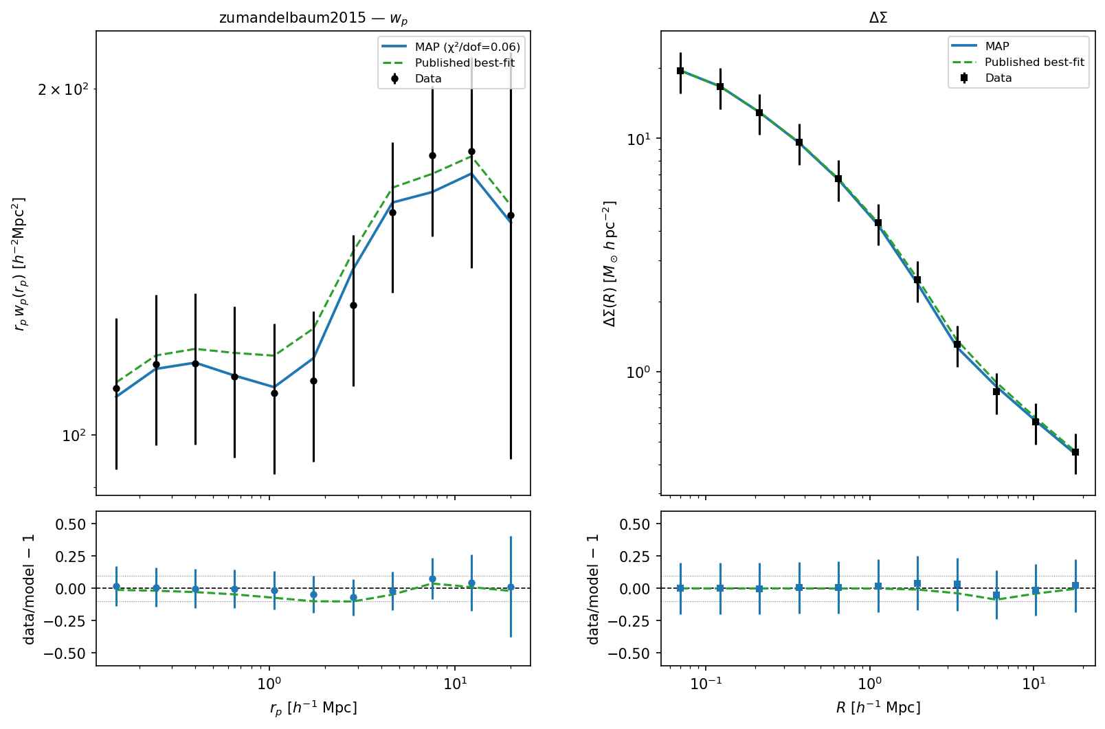
MAP fit to SDSS DR7 \(\log_{10}(M_*/h^{-2}M_\odot) > 10.2\). Top: \(w_p(r_p)\). Bottom: \(\Delta\Sigma(R)\).
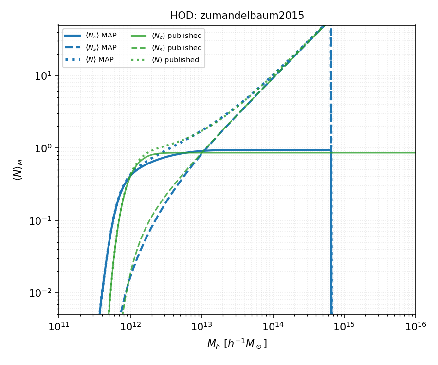
HOD occupation functions vs halo mass at the MAP parameters.
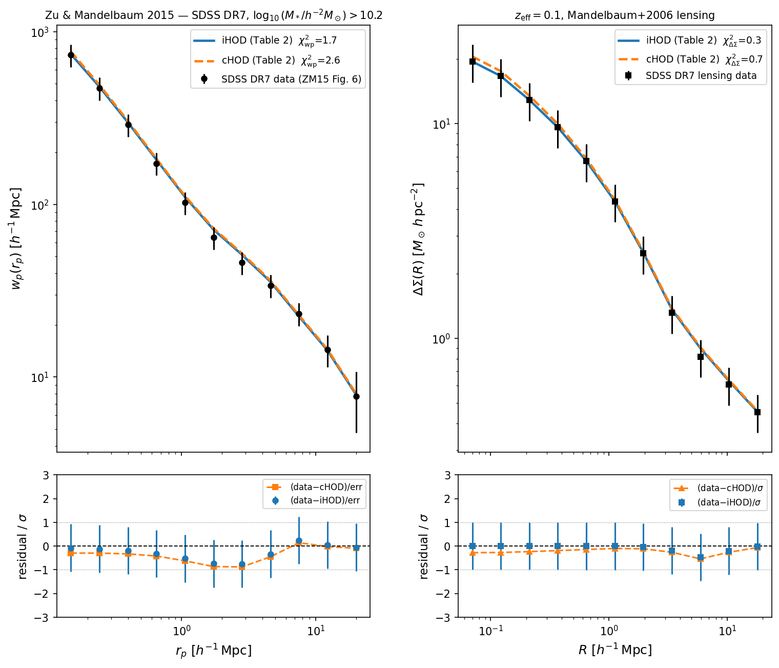
Comparison of iHOD (ZuMandelbaum15) and cHOD (conventional) predictions for \(w_p\) and \(\Delta\Sigma\). Differences are at the 1–2% level — both approaches produce statistically equivalent predictions for these observables.
For the 7-bin multi-sample iHOD fit (all stellar-mass bins simultaneously, joint \(\chi^2/\mathrm{dof} = 2.34\)), see Benchmark: Zu & Mandelbaum 2015 — Multi-Sample iHOD.
X-ray cross-correlation extension
For the BGS × eROSITA analysis (Comparat et al. 2025, arXiv:2503.19796), the ZM15 iHOD is extended with a gas density component and an AGN component.
Gas density profile (GasDensityDPM)
Reference: Oppenheimer et al. 2025
(arXiv:2505.14782),
implemented in GasDensityDPM.
The electron density profile uses a generalised NFW shape (arXiv:2505.14782 Eq. 1):
where \(x = r/R_s\) and \(R_s = R_{200}/c(M,z)\).
The concentration \(c(M,z)\) follows Diemer & Joyce 2019
(arXiv:1809.07326),
via c_diemer15(),
the same relation used for the NFW galaxy profile.
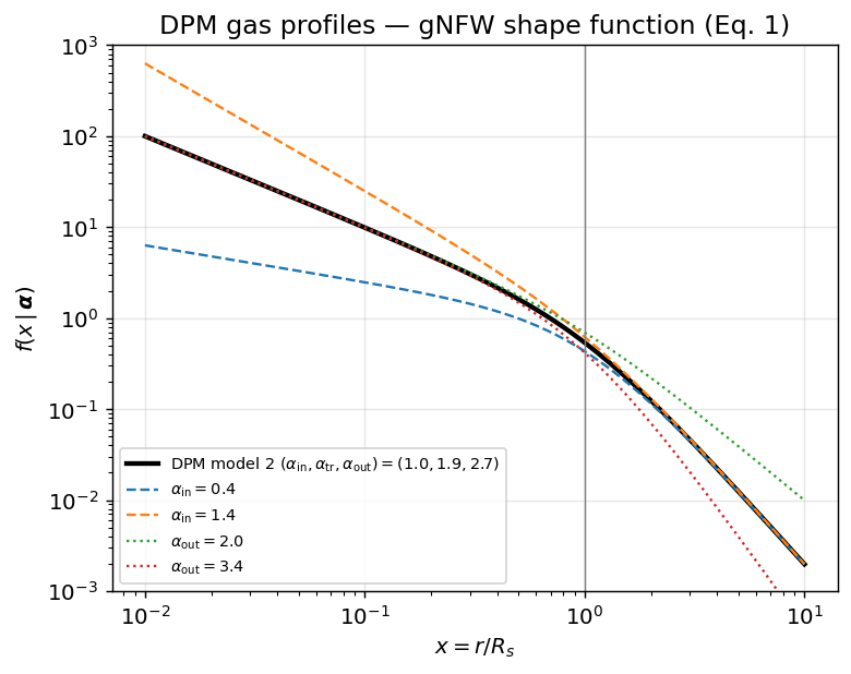
gNFW shape function \(f(x|\boldsymbol{\alpha})\) shared by all three DPM profiles, varying the inner and outer slopes. Cosmology-independent.
The electron density (arXiv:2505.14782 Eq. 3):
Default model 2 parameters (Table 1 of arXiv:2505.14782): \(n_{e,0.3} = 4.87 \times 10^{-5}\) cm-3, \(\alpha_\mathrm{in} = 1.0\), \(\alpha_\mathrm{tr} = 1.9\), \(\alpha_\mathrm{out} = 2.7\), \(\beta_\mathrm{gas} = 0.36\) (mass slope; free in fitting), \(\gamma = 2.0\).
Gas pressure profile (PressureProfileDPM)
The electron pressure uses the same gNFW shape with mass-dependent outer slope (arXiv:2505.14782 Eq. 5) and mass/redshift scaling (Eq. 2):
Model 2 parameters: \(P_{0.3} = 115\) meV cm-3, \(\beta^P = 0.85\), \(\gamma^P = 8/3\).
Gas metallicity profile (MetallicityProfileDPM)
A gNFW metallicity profile (no mass or redshift dependence):
with \(\alpha^Z_\mathrm{in}=0\), \(\alpha^Z_\mathrm{tr}=0.5\), \(\alpha^Z_\mathrm{out}=0.7\) (Table 1 of arXiv:2505.14782).
X-ray emissivity — APEC cooling function
All three DPM profiles are evaluated at every Gauss-Legendre quadrature node. The temperature at radius \(r\) is derived from the ideal gas law:
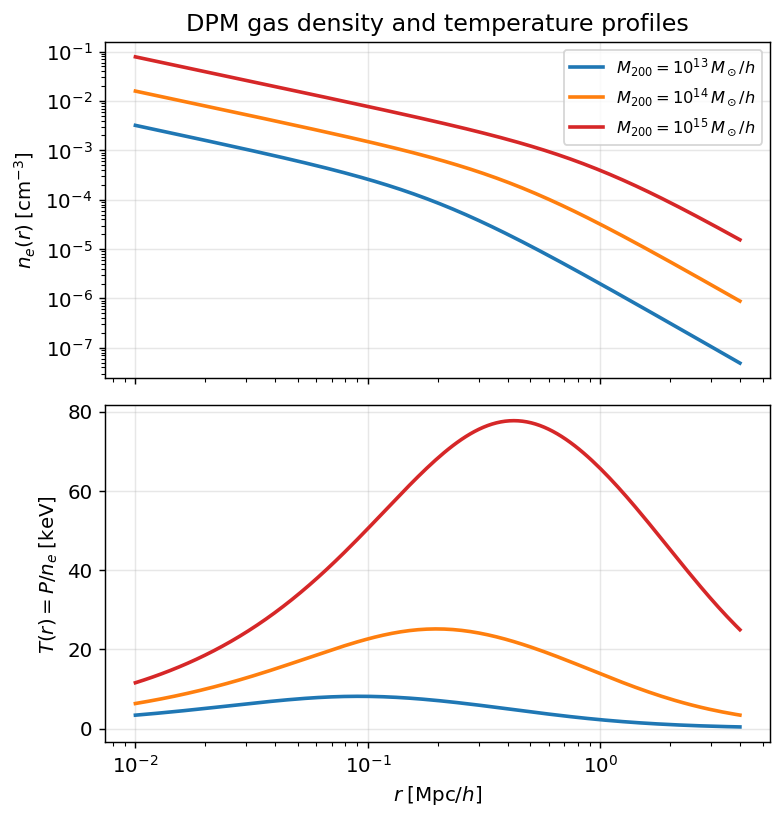
DPM electron density \(n_e(r)\) (top) and temperature \(T(r)=P/n_e\) (bottom) for three halo masses, showing the \(M_{12}^{\beta}\) mass scaling. Cosmology-independent (fixed cosmology).
The 0.5–2 keV soft X-ray emissivity per unit volume is:
where \(\Lambda_{n_e^2}(T, Z) = 0.83\,\Lambda_{\rm APEC}(T, Z)\) is
the band-integrated APEC cooling function (AtomDB, via soxs + pyXSIM), precomputed over a
log-spaced \((T, Z)\) grid at initialisation and evaluated by 2D
log-log interpolation at runtime
(ApecCoolingTable).
The factor 0.83 converts from the \(n_e n_H\) APEC convention to
\(n_e^2\) (\(n_H \approx 0.83\,n_e\) for solar-abundance plasma).
Reference values (0.5–2 keV, AtomDB 3.1.3, abund_table="angr"):
\(T\) [keV] |
\(Z\) [\(Z_\odot\)] |
\(\Lambda_{n_e^2}\) [erg cm3 s-1] |
|---|---|---|
0.5 |
0.3 |
\(\approx 8.0\times10^{-24}\) |
1.0 |
0.3 |
\(\approx 7.6\times10^{-24}\) |
2.0 |
0.3 |
\(\approx 5.0\times10^{-24}\) |
1.0 |
1.0 |
\(\approx 1.9\times10^{-23}\) |
An overall amplitude \(A_\mathrm{gas}\) is a free parameter fitted jointly with the HOD parameters.
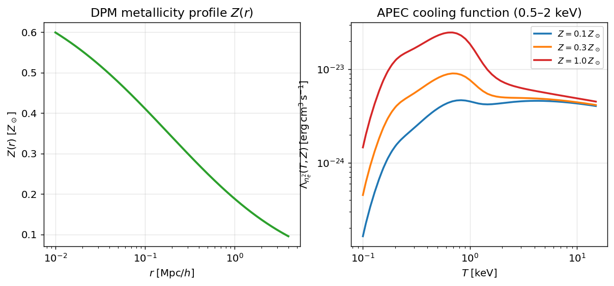
Left: the gNFW metallicity profile \(Z(r)\). Right: the band-integrated APEC cooling function \(\Lambda_{n_e^2}(T,Z)\) (0.5–2 keV, AtomDB) vs temperature for three metallicities. Cosmology-independent.
HAM AGN model (HamAGNModel)
References: Aird et al. 2015, ApJ 815, 66
(arXiv:1503.01120) — LADE hard XLF;
Comparat et al. 2019, A&A 622, A12
(arXiv:1901.10866) — obscuration model;
implemented in HamAGNModel.
The HAM pipeline assigns a hard X-ray luminosity to each halo by abundance-matching the cumulative halo number density (from the iHOD SHMR) to the cumulative AGN number density from the Aird+2015 LADE hard XLF.
LADE hard XLF (Aird+2015, 2–10 keV):
with luminosity-dependent density evolution (LADE):
and slopes \(\gamma_1 = 0.48\), \(\gamma_2 = 2.27\) (Comparat+2019 eqs. 2–3 fit to Aird+2015).
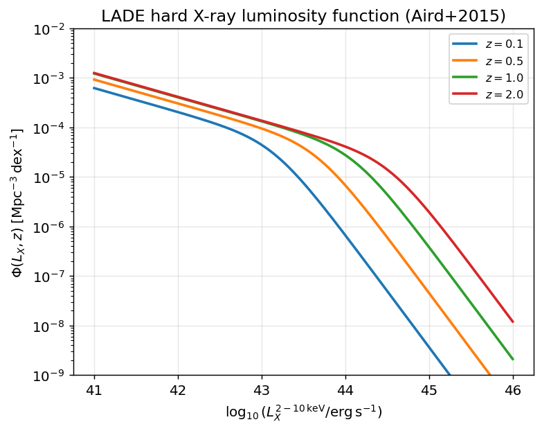
LADE hard X-ray luminosity function \(\Phi(L_X,z)\) (Aird+2015) at four redshifts, showing the luminosity-dependent density evolution.
Abundance matching: at each \((M_h, z)\), the iHOD cumulative number density \(n_\mathrm{gal}(>M_*(M_h), z)\) multiplied by the AGN duty cycle \(f_\mathrm{DC}(z)\) is matched to \(n_\mathrm{AGN}(>L_X, z)\) from the XLF, yielding \(\langle L_X^\mathrm{hard}(M_h, z)\rangle\). This table is precomputed at initialisation on a 2D \((z, M_h)\) grid.
Duty cycle \(f_\mathrm{DC}(z)\):
\(z\) |
\(f_\mathrm{DC}\) |
|---|---|
0.00 |
0.038 |
0.25 |
0.097 |
0.75 |
0.40 |
\(\geq 1.75\) |
0.50 |
Obscuration model (Comparat+2019 eqs. 4–11):
Compton-thick luminosity threshold — the CT boundary shifts with redshift:
Compton-thick fraction (log \(N_H \geq 24\), Comparat+2019 eq. 4):
Bright-end obscured fraction (Comparat+2019 eq. 5) — floor from CT plus a redshift-dependent boost:
Faint-end obscured fraction (Comparat+2019 eq. 6) — rising toward low luminosities:
Transition luminosity (crossover between the two regimes):
Blending weight (smooth interpolation between \(f_1\) and \(f_2\)):
Total obscured fraction (log \(N_H > 22\), type-2 + CT, Comparat+2019 eq. 11):
Type fractions derived from \(f_\mathrm{obsc}\) and \(f_{CT}\):
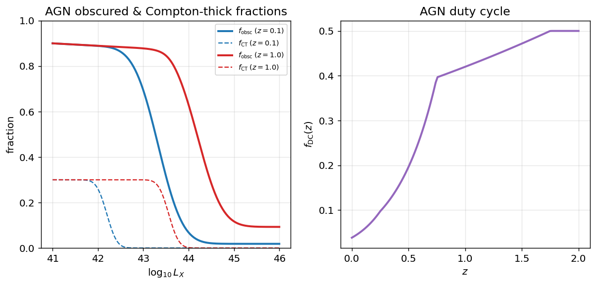
Left: AGN obscured (\(\log N_H>22\)) and Compton-thick fractions vs \(\log L_X\) at two redshifts. Right: the AGN duty cycle \(f_\mathrm{DC}(z)\). Cosmology-independent.
Hard-to-soft conversion: the effective K-correction is averaged over the
three type classes using the precomputed absorption table
(hod_mod/data/agn/v3_fraction_observed_A15_RF_hard_Obs_soft_fscat_002.txt,
generated by integrating an absorbed power-law with \(\Gamma=1.9\) and
\(f_\mathrm{scat}=0.02\) over a \(35\times16\) grid of
\((z,\log N_H)\) values):
The hard-to-soft ratio for unobscured AGN at \(z=0\) is 0.607.
Mean soft X-ray luminosity: combining HAM hard luminosity, K-correction, duty cycle, and log-normal scatter boost:
with log-normal scatter \(\sigma_\mathrm{dex} = 0.8\) dex in \(L_X\) at fixed \(M_h\).
AGN are unresolved point sources, so their angular template is the PSF (King profile, \(\theta_c = 8.64\) arcsec on-axis eROSITA):
Prediction pipeline — from profiles to \(w_\theta(\theta)\)
The six steps below go from the DPM profile parameters to the observable
angular cross-correlation. All steps are implemented in
HaloModelCrossSpectra.
Step 1 — Emissivity profile Fourier transform \(\tilde{X}(k|M,z)\)
The key quantity linking the 3D profile to the halo model is the spherical
Fourier transform of the per-halo emissivity (implemented in
emissivity_full_uk()):
where \(j_0(x) = \sin(x)/x\).
\(T(r) = P(r)/n_e(r)\) [keV] from the ideal gas law (Step 1 of
temperature_from_profiles()).
The radial integral uses 200-point Gauss-Legendre quadrature up to
\(r_\mathrm{max} = 3\,R_{200}\).
At \(k \to 0\), \(\tilde{X}(0|M,z)\) equals the total halo emissivity \(L_X^\mathrm{gas}(M,z)/\Lambda_\mathrm{ref}\) in volume units \([\mathrm{Mpc}/h]^3\,\mathrm{cm}^{-6}\).
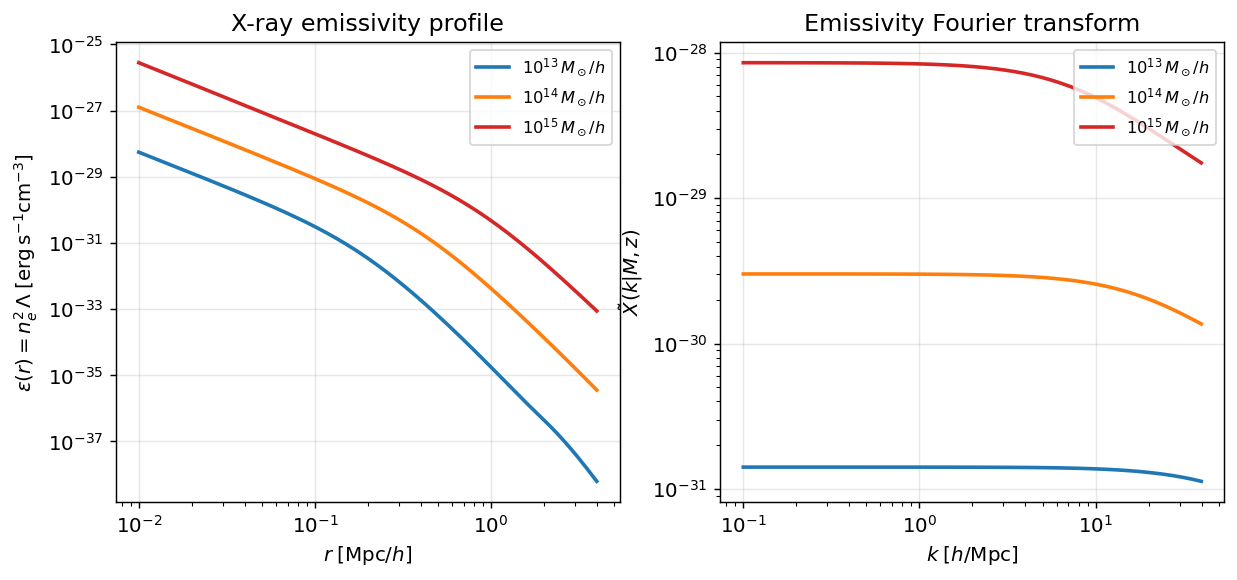
Left: X-ray emissivity profile \(\varepsilon(r)=n_e^2\,\Lambda(T,Z)\) for three halo masses. Right: the spherical Fourier transform \(\tilde X(k|M,z)\) that links the 3D emissivity to the halo model.
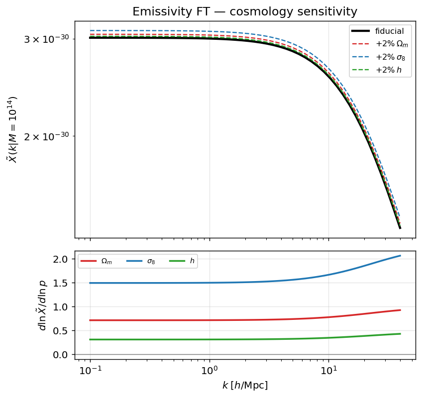
Cosmology sensitivity of the emissivity Fourier transform \(\tilde X(k|M)\) at \(M_{200}=10^{14}\,M_\odot/h\). Lower panel: the logarithmic sensitivity \(d\ln\tilde X/d\ln p\) to \(\Omega_m\), \(\sigma_8\) and \(h\) (through the concentration and \(E(z)\) scaling; central finite differences) — the cosmology dependence that propagates into \(P_{gX}\), \(C_\ell^{gX}\) and \(w_\theta\).
Step 2 — 3D galaxy × X-ray power spectrum \(P_{gX}(k,z)\)
The halo model splits \(P_{gX}\) into 1-halo and 2-halo contributions
(_pk_tables_gX()):
1-halo term (galaxies and X-ray emission in the same halo):
where \(\tilde{u}(k|M)\) is the NFW dark-matter profile Fourier transform,
and \(N_c,\,N_s\) are the central/satellite occupation from
ZuMandelbaum15HODModel.
2-halo term (galaxies in one halo, X-ray emission from a different halo, correlated by large-scale structure):
The total is \(P_{gX} = P_{gX}^{1h} + P_{gX}^{2h}\).
Note on 1-halo vs 2-halo amplitude
At angular scales \(\theta \in [8'',\,300'']\) (i.e. \(k \approx 1.3\)–\(49\,h\,\mathrm{Mpc}^{-1}\) at \(z=0.135\)), the 1-halo term dominates the prediction by factors of 9–12 000 over the 2-halo term. Both terms are computed in full; the 2-halo only overtakes the 1-halo at \(\theta \gtrsim 1^\circ\) (outside the data range).
The predicted \(w_\theta(\theta)\) can appear “2-halo-like” (a smooth power-law slope) because the dominant signal traces the outer gNFW profile at \(r > R_{200}\) (where \(\alpha_\mathrm{out}=2.7\) gives \(n_e^2 \propto r^{-5.4}\), a steep power law), plus the contribution of satellite galaxies sitting in X-ray bright clusters.
Step 3 — Mass-slope tilt (free parameters \(\beta_\mathrm{gas}\), \(\beta_P\))
After computing \(\tilde{X}\) at the DPM reference slopes, two multiplicative tilts are applied in mass space (no re-integration needed):
with \(\beta_\mathrm{gas}^0 = 0.36\) and \(\beta_P^0 = 0.85\) (DPM model 2). These replace full re-integration and make the fitting fast (cached \(\tilde{X}\) reused across MCMC steps).
Step 4 — X-ray window function \(W_X(\chi)\) and Limber integral
The galaxy × X-ray cross-spectrum via the Limber approximation (Loverde & Afshordi 2008, arXiv:0809.5112):
There is no separate \(W_X(\chi)\) window function. The X-ray emissivity response is entirely encoded in \(P_{gX}(k,z)\) via \(\tilde{X}(k|M,z)\): the halo model automatically integrates the emissivity profile over all halos at each redshift. Symbolically, writing \(W_X(\chi) = \langle\varepsilon(z)\rangle/\langle S_X\rangle\) would require knowing the mean background emissivity; instead the halo model computes \(P_{gX}\) directly, bypassing that normalisation.
The Limber integrand is evaluated on a grid of \(N_z\) redshift slices spanning the galaxy \(n_g(z)\), with \(k_\mathrm{Limber} = (\ell + \tfrac{1}{2})/\chi(z)\). The \(\ell\) grid spans \(\ell \in [10,\,10^5]\) on 160 log-spaced points; \(\ell_\mathrm{max} = 10^5\) resolves \(\theta = 8''\) (\(\ell \approx 25\,800\) at \(z_\mathrm{mean} = 0.135\)).
Step 5 — PSF convolution
The gas \(C_\ell^{gX}\) is multiplied by the eROSITA PSF window in \(\ell\)-space (King profile, \(\theta_c = 8.64''\), \(\alpha = 1.5\)):
where \(K_\nu\) is the modified Bessel function and \(C\) normalises \(B_0 = 1\). At \(\ell = 25\,800\) (\(\theta_c = 8.64'' = 4.19\times10^{-5}\,\mathrm{rad}\)), \(\ell\,\theta_c \approx 1.08\) so \(B_\ell \approx 0.5\): the PSF suppresses but does not eliminate signal at \(\theta = 8''\).
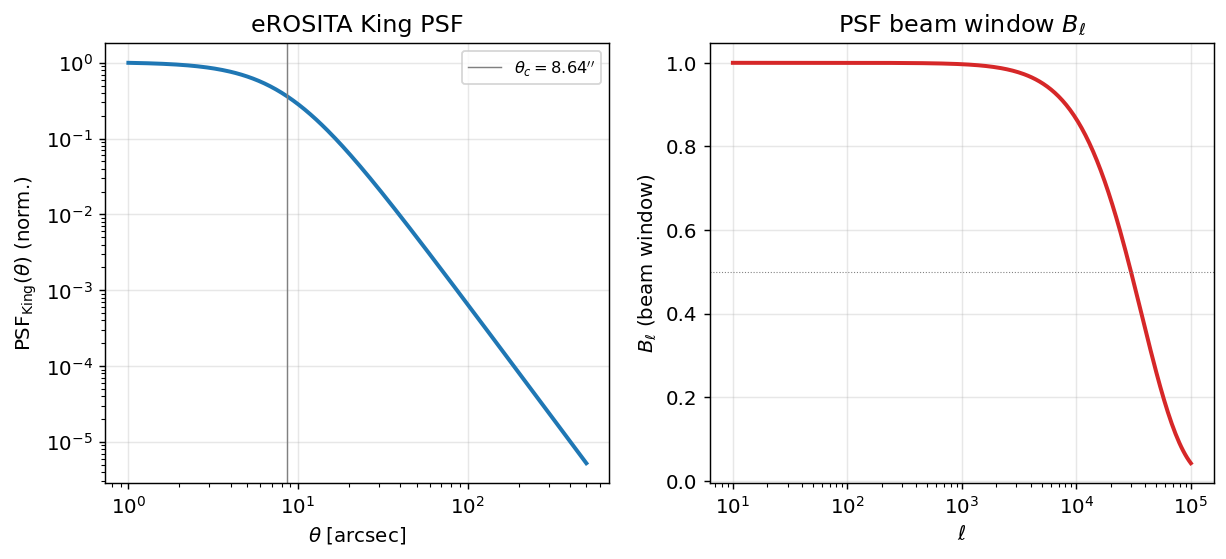
Left: the eROSITA King PSF \(\mathrm{PSF}_\mathrm{King}(\theta)\). Right: the corresponding beam window \(B_\ell\) that multiplies the gas \(C_\ell^{gX}\). Instrument response — cosmology-independent.
Step 6 — Angular correlation function and full model
The PSF-convolved \(C_\ell\) is Hankel-transformed to the angular correlation function:
The full model at the 31 data bins \(\theta \in [8'',\,300'']\) is:
where \(s_\mathrm{gas}(\theta)\) is the Hankel transform of \(C_\ell^\mathrm{gas}\) (both 1h and 2h included), and \(A_\mathrm{gas}\),,:math:A_mathrm{AGN} are free dimensionless amplitudes. AGN are treated as unresolved point sources so their template is \(\mathrm{PSF}_\mathrm{King}(\theta)\) directly (no halo-model \(C_\ell^{gX,\mathrm{AGN}}\)), avoiding a spurious 2-halo hump at large \(\theta\) in the AGN component.
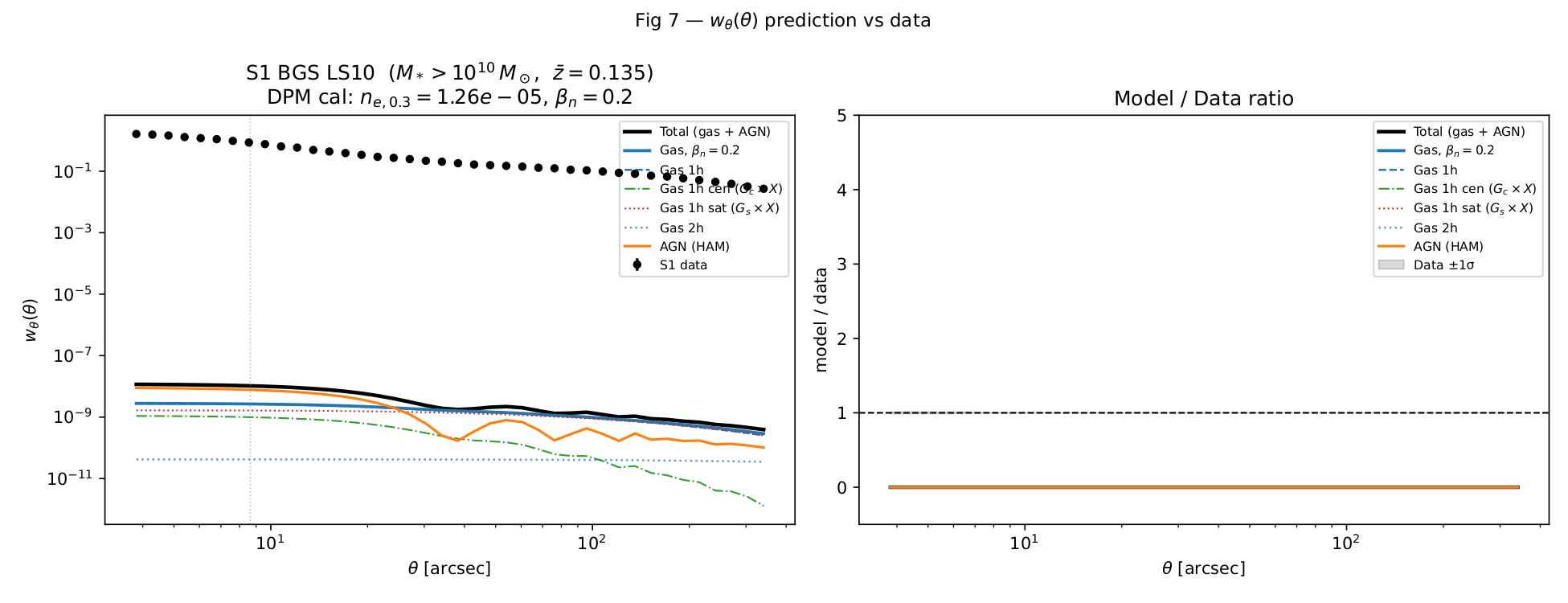
Angular cross-correlation \(w_\theta(\theta)\) for BGS S1 (\(\log_{10}M_* > 10\), \(z_\mathrm{mean} = 0.135\)). Gas (blue), AGN (orange), and total (black) model components vs eROSITA data (grey).
BGS X-ray fit parameters (8 free parameters)
Parameter |
Symbol |
Prior range |
Units |
Description |
|---|---|---|---|---|
|
\(\log_{10} A_\mathrm{gas}\) |
\([-2,\,12]\) |
— |
gas amplitude (absorbs \(\Lambda_\mathrm{eff}\) and unit conversion) |
|
\(\beta_\mathrm{gas}\) |
\([0,\,0.8]\) |
— |
gas density mass slope (overrides DPM calibrated value) |
|
\(\beta_P\) |
\([0,\,2]\) |
— |
pressure profile mass slope (for future tSZ extension) |
|
\(\log_{10} A_\mathrm{AGN}\) |
\([-5,\,15]\) |
— |
AGN amplitude (absorbs duty cycle and unit conversion) |
|
\(\log_{10} M_{*,\mathrm{th}}\) |
\([9,\,12]\) |
\(\log_{10}(M_\odot)\) |
stellar-mass threshold of the BGS sample |
|
\(\sigma_{\ln M_*}\) |
\([0.01,\,1.5]\) |
— |
scatter in \(\ln M_*\) at fixed \(M_h\) |
|
\(\log_{10} M_1\) |
\([9.5,\,14]\) |
\(\log_{10}(M_\odot h^{-1})\) |
SHMR pivot halo mass |
|
\(\alpha_\mathrm{sat}\) |
\([0.5,\,2.5]\) |
— |
satellite occupation power-law slope |
All SHMR shape parameters (\(\beta,\,\delta,\,\gamma,\,\eta,\,f_c,\,B_\mathrm{sat}\)) are held at their ZM15 published best-fit values during BGS fitting.
Complete model parameter inventory
The table below covers every named parameter of the three model components. Column Status uses: Free = fitted in the BGS 8-parameter run; Fixable = currently fixed but physically meaningful to free; Fixed = hard-coded or calibrated from simulation / external data.
Parameter / symbol |
Value |
Status |
Component |
Notes |
|---|---|---|---|---|
\(\log_{10} A_\mathrm{gas}\) |
(fitted) |
Free |
Gas |
Amplitude of the emissivity template; absorbs overall normalisation uncertainty |
\(\beta_\mathrm{gas}\) ( |
(fitted) |
Free |
Gas |
Mass slope of \(n_e\); overrides DPM model-2 calibrated value 0.36 |
\(\beta_P\) ( |
(fitted) |
Free |
Gas |
Mass slope of pressure profile; sets \(T(r) \propto M^{\beta_P - \beta_n}\) at fixed shape |
\(\log_{10} A_\mathrm{AGN}\) |
(fitted) |
Free |
AGN |
Amplitude of the AGN PSF template; absorbs duty-cycle and unit-conversion uncertainty |
\(\log_{10} M_{*,\mathrm{th}}\) ( |
10.0 (S1) |
Free |
iHOD |
Stellar-mass threshold; determines effective \(M_\mathrm{min}\) of the sample |
\(\sigma_{\ln M_*}\) ( |
0.50 |
Free |
iHOD |
SHMR scatter; controls satellite richness and the width of the 1-halo gas peak |
\(\log_{10} M_1\) ( |
12.10 |
Free |
iHOD |
SHMR pivot halo mass; sets \(\langle M_h\rangle\) of the galaxy sample |
\(\alpha_\mathrm{sat}\) ( |
1.00 |
Free |
iHOD |
Satellite occupation slope; affects the 2-halo to 1-halo transition |
\(n_{e,0.3}\) ( |
\(4.87\times10^{-5}\ \mathrm{cm}^{-3}\) |
Fixable |
Gas |
Density amplitude at \(0.3\,R_{200}\) (degenerate with \(A_\mathrm{gas}\); freeing it would allow a physical normalisation) |
\(P_{0.3}\) |
\(115\ \mathrm{meV\,cm}^{-3}\) |
Fixable |
Gas |
Pressure amplitude; sets \(T \propto P/n_e\); freeing it changes the spectral shape via \(\Lambda_\mathrm{APEC}(T, Z)\) |
\(\alpha_\mathrm{out}\) (density) |
2.7 |
Fixable |
Gas |
Outer gNFW slope; controls how quickly the gas profile truncates beyond \(R_{200}\) |
\(Z_0\) (metallicity amplitude) |
\(Z(0.3\,R_{200}) = 0.3\,Z_\odot\) |
Fixable |
Gas |
Normalisation of the metallicity profile; shifts \(\Lambda_\mathrm{APEC}\) by ~30% if doubled |
\(\sigma_\mathrm{dex}\) (AGN scatter) |
0.8 |
Fixable |
AGN |
Log-normal scatter in \(L_X\) at fixed \(M_h\); partly degenerate with \(A_\mathrm{AGN}\) |
\(f_\mathrm{sat,AGN}\) |
0.10 |
Fixable |
AGN |
Fraction of satellite galaxies hosting AGN; affects the angular scale dependence of the AGN term |
\(\log_{10} M_{*,0}\) ( |
10.31 |
Fixed (ZM15) |
iHOD |
SHMR pivot stellar mass; held at ZM15 Table 2 value |
\(\beta\) ( |
0.33 |
Fixed (ZM15) |
iHOD |
Low-mass SHMR power-law slope |
\(\delta\) ( |
0.42 |
Fixed (ZM15) |
iHOD |
High-mass SHMR transition exponent |
\(\gamma\) ( |
1.21 |
Fixed (ZM15) |
iHOD |
High-mass SHMR power-law slope |
\(\eta\) ( |
−0.04 |
Fixed (ZM15) |
iHOD |
Mass-dependent scatter slope |
\(f_c\) ( |
0.86 |
Fixed (ZM15) |
iHOD |
Central galaxy fraction |
\(B_\mathrm{sat}\) ( |
8.98 |
Fixed (ZM15) |
iHOD |
Satellite halo-mass normalisation |
\(\beta_\mathrm{sat}\), \(\beta_\mathrm{cut}\) |
0.90, 0.41 |
Fixed (ZM15) |
iHOD |
Satellite and cut-off mass-scaling slopes |
\(B_\mathrm{cut}\) ( |
0.86 |
Fixed (ZM15) |
iHOD |
Central cut-off normalisation |
\(\alpha_\mathrm{in},\,\alpha_\mathrm{tr}\) (density) |
1.0, 1.9 |
Fixed (DPM) |
Gas |
Inner slope and transition steepness of the gNFW density profile |
\(\gamma_n\) (density redshift) |
2.0 |
Fixed (DPM) |
Gas |
Redshift scaling exponent \(E(z)^{\gamma_n}\) |
\(\gamma^P,\,\alpha^P_\mathrm{out}(M)\) |
8/3, mass-dep. |
Fixed (DPM) |
Gas |
Pressure profile redshift slope and (mass-dependent) outer slope |
\(\alpha^Z_\mathrm{in},\,\alpha^Z_\mathrm{tr},\,\alpha^Z_\mathrm{out}\) |
0, 0.5, 0.7 |
Fixed (DPM) |
Gas |
Metallicity profile shape parameters |
\(f_\mathrm{DC}(z)\) (duty cycle table) |
0.038–0.50 |
Fixed (C19) |
AGN |
AGN duty cycle at six redshift nodes (Comparat+2019 Table 3) |
Obscuration constants (\(L_{ll}\), \(f_{CT}\), etc.) |
see eqs. above |
Fixed (C19) |
AGN |
All numerical constants in Comparat+2019 eqs. 4–11 |
K-correction table (\(k(z, N_H)\)) |
precomputed |
Fixed (C19) |
AGN |
Absorbed power-law (\(\Gamma=1.9,\,f_\mathrm{scat}=0.02\)) integrated over \(35\times16\) grid |
\(c(M,z)\) concentration |
Diemer+2019 |
Fixed |
Gas |
Diemer & Joyce 2019 mass–concentration relation used for all gas profiles |
Fixed-ZM15 X-ray fit — AGN + gas model options
The galaxy sector (ZM15 iHOD) and the X-ray sector (gas + AGN) can be fit
separately. Rather than floating the 8 galaxy+X-ray parameters jointly
against \(w_\theta + w_p + \Phi(M_*)\) (previous section), the
stellar–halo connection is taken as already determined by the dedicated
\(w_p + \bar n_g\) joint fit
(hod_mod.scripts.fitting.bgs_ls10.fit_bgs_zm15_joint), held fixed,
and only the X-ray/gas/AGN parameters are fit against the galaxy × eROSITA
cross-correlation \(w_\theta(\theta)\). This is enabled by
fit_comparat2025 --fix-zm15 and isolates what the X-ray data constrain,
free of the galaxy–X-ray parameter degeneracies.
Fixed galaxy parameters — \(w_p + \bar n_g\) joint MAP fit
Source: results/bgs_zm15_joint_wp_ngal/map_result.json
(hod_mod.scripts.fitting.bgs_ls10.fit_bgs_zm15_joint, --mode map,
8 stellar-mass bins \(10.0 \le \log_{10}M_* < 12.0\),
\(w_p(r_p) + \bar n_g\), no lensing). Joint
\(\chi^2/\mathrm{dof} = 44.03/99 = 0.445\).
Note
This is the frozen June-2026 reference MAP, not the v0.3 campaign fit of
the same model. It is deliberately held fixed — _campaign_env.sh
symlinks it into every versioned results tree as a REFERENCE_INPUTS
entry — so that the Family-C X-ray presets stay comparable across campaigns.
The v0.3 re-fit of the same data is a different run with
\(\chi^2/\mathrm{dof} = 59.70/99 = 0.603\) and a noticeably different
posterior; see BGS × LS10 — Zu & Mandelbaum 2015 joint w_p + n_{\rm gal} MCMC. Do not mix the two.
All 13 parameters below are held fixed when running --fix-zm15; the
stellar-mass threshold \(\log_{10}M_{*,\mathrm{th}}\) is set per sample
(10.0 for S1, overridable with --zm15-thresh).
Parameter |
MAP value |
ZM15 Table 2 |
Component / role |
|---|---|---|---|
|
11.900 |
\(12.10\pm0.17\) |
SHMR pivot halo mass |
|
10.367 |
\(10.31\pm0.10\) |
SHMR pivot stellar mass |
|
0.426 |
\(0.33\pm0.21\) |
low-mass SHMR slope |
|
0.616 |
\(0.42\pm0.04\) |
high-mass SHMR transition exponent |
|
1.686 |
\(1.21\pm0.20\) |
high-mass SHMR slope |
|
0.823 |
\(0.50\pm0.04\) |
scatter in \(\ln M_*\) at fixed \(M_h\) |
|
−0.227 |
\(-0.04\pm0.02\) |
mass-dependent scatter slope |
|
0.754 |
\(0.86\pm0.14\) |
central completeness fraction |
|
17.544 |
\(8.98\pm1.18\) |
satellite halo-mass normalisation |
|
0.493 |
— |
satellite mass-scaling slope |
|
9.634 |
— |
cut-off normalisation |
|
0.820 |
— |
cut-off mass-scaling slope |
|
1.250 |
— |
satellite occupation slope |
AGN + gas model — free-parameter options
With ZM15 fixed, the X-ray sector is fit against \(w_\theta\)
alone (\(w_p\) and \(\Phi(M_*)\) no longer depend on any free
parameter, so they are shown as fixed-prediction diagnostic overlays). The
free X-ray/gas/AGN parameters are selected with --free-params:
Preset |
N |
Free parameters |
Notes |
|---|---|---|---|
|
2 |
\(\log_{10}A_\mathrm{gas},\ \log_{10}A_\mathrm{AGN}\) |
gas slopes fixed (\(\beta_\mathrm{gas}=0.25,\ \beta_P=0.86\)) |
|
3 |
\(\log_{10}A_\mathrm{gas},\ \beta_\mathrm{gas},\ \beta_P\) |
AGN amplitude fixed |
|
4 |
\(\log_{10}A_\mathrm{gas},\ \beta_\mathrm{gas},\ \beta_P,\ \log_{10}A_\mathrm{AGN}\) |
amplitude + mass-tilt model (cheap) |
|
6 |
|
DPM profile shapes; rebuilds the gas profiles per eval (slow) |
|
8 |
|
|
|
14 |
|
every DPM gas parameter |
|
4 |
\(\log_{10}A_\mathrm{gas},\ \beta_\mathrm{gas},\ \beta_P,\ \log_{10}A_\mathrm{AGN}\) |
= |
|
7 |
|
HamAGNModel luminosity overrides (needs |
|
8 |
|
HODAgnModel occupation (needs |
An explicit subset of registry names may also be passed, e.g.
--free-params log10_A_gas beta_gas alpha_out_gas.
Cost and identifiability (w_θ-only fit)
The gas-* presets rebuild the DPM gas profiles per likelihood
evaluation (seconds each) and switch on the full APEC emissivity path
(\(\varepsilon = n_e^2\,\Lambda(T,Z)\)) so the pressure/temperature/
metallicity parameters take effect. Because the likelihood is \(w_\theta\)
only, the shape parameters (gas \(\alpha\)/\(\beta\) slopes)
reshape the prediction, but the
normalisation parameters (\(n_{e,0.3}\)) and the agn-lum AGN-luminosity
parameters are degenerate with \(\log_{10}A_\mathrm{gas}/\log_{10}A_\mathrm{AGN}\)
— they run as flat directions and stay near their seeds. They are exposed for
forward-modelling, priors and a future multi-probe (X-ray luminosity) fit.
AGN + gas model — component choices
Option |
Class |
Behaviour |
|---|---|---|
|
|
A physically predicted, occupation-weighted AGN cross-power, convolved
with the PSF inside |
|
|
Flux-selected variant of the occupation model, used for the
|
|
The AGN is an unresolved point source, so its angular template is the eROSITA King PSF (\(\theta_c = 8.64''\)) and the fit varies only its amplitude \(\log_{10}A_\mathrm{AGN}\), which sets the whole AGN flux scale. |
|
|
ZuMandelbaum15 occupation (fixed from the \(w_p+\bar n_g\) MAP fit) \(\times\) a free duty cycle \(10^{\log_{10}DC}\), with the \(W_\mathrm{AGN}(z)\) X-ray-flux kernel (Eq. A9). The duty cycle is the only free AGN parameter. See the dedicated section below. |
The gas component is the DPM model-2 stack in every case
(GasDensityDPM +
PressureProfileDPM + MetallicityProfileDPM +
ApecCoolingTable). By default only the
\(\beta_\mathrm{gas}\)/\(\beta_P\) mass-slope tilts (Step 3 above) are
free; the gas-shape/gas-temp/gas-full presets additionally expose the
gNFW profile shapes, normalisations and metallicity (see the preset table above).
Running the fixed-ZM15 fit
# full gas + AGN X-ray model (4 free params), S1 = M* > 10
JAX_PLATFORMS=cpu python -m hod_mod.scripts.fitting.fit_comparat2025 \
    --sample S1 --fix-zm15 --mode map --free-params all

# two amplitudes only (gas slopes fixed)
JAX_PLATFORMS=cpu python -m hod_mod.scripts.fitting.fit_comparat2025 \
    --sample S1 --fix-zm15 --mode map --free-params amps

# richer DPM gas profile (slow: full APEC path, profile rebuild per eval)
JAX_PLATFORMS=cpu python -m hod_mod.scripts.fitting.fit_comparat2025 \
    --sample S1 --fix-zm15 --mode map --free-params gas-shape \
    --out-dir results/fits/comparat2025_fixedZM15_gas-shape

# free-amplitude King PSF AGN at fixed gas (PSF-amplitude model)
JAX_PLATFORMS=cpu python -m hod_mod.scripts.fitting.fit_comparat2025 \
    --sample S1 --fix-zm15 --mode map --free-params agn-models --agn-model ham \
    --out-dir results/fits/comparat2025_fixedZM15_agn-models_ham
Results (MAP json + best-fit / diagnostics / gas-diagnostics figures) are
written to results/fits/comparat2025_fixedZM15/ (overridable per run with
--out-dir) — separate from the joint-fit results/fits/comparat2025/ so
neither clobbers the other.
The --ecf runs of the v0.4 campaign are invalid
--ecf (0.4.0) folds the validated eROSITA flux→count ECF into both legs
and anchors the residual amplitudes on S1. In the VTAG=v0.4 campaign the
anchor was measured by a non-negative solve under a weighting that drove
the AGN conversion negative, so it clipped to exactly zero — and since the
model applies it as A_AGN = 10**log10_A_AGN * c_agn, every --ecf fit
ran with no AGN component at all.
An earlier revision of this page attributed the identical \(\log_{10}A_\mathrm{AGN} = -3.3139\) reported by four presets to the amplitude railing against a bound. That was wrong: the range is \((-5, 15)\) and the value is interior. It is the optimiser’s seed, returned untouched because a zero conversion makes the direction exactly flat.
The anchor is fixed (likelihood-consistent weights, unconstrained solve, and
a degenerate anchor now raises rather than being cached), but the five
--ecf presets have not yet been re-run. Full diagnosis, the
goodness-of-fit tables and the cross-campaign comparison are on
Family C — fixed-ZM15 X-ray w(\theta) preset fits.
Diagnostic SMF/n_gal units (h³)
The _diagnostics.pdf stellar-mass-function and \(\bar n_g\) panels
compare the model (native \((\mathrm{Mpc}/h)^{-3}\)) against the sum_stat
SMF. The raw HDF5 phi is in physical \(\mathrm{Mpc}^{-3}\), so
load_smf_data divides it by \(h^3\) (as
smf() does) before
plotting — without this the panels read \(\sim h^{-3}\approx3.2\times\) too
high. With the fixed ZM15 parameters the model then reproduces the SMF and
\(\bar n_g\) (ratio \(\approx1\)); only the high-mass tail
(\(\log_{10}M_*\gtrsim11.5\)) is over-predicted, the known iHOD limitation.
Note
The table below is an older --free-params all run and carries no campaign
tag — it is not one of the ten v0.4 Family-C fits. For campaign-tagged
results, the five presets side by side, and the v0.3/v0.31/v0.4 comparison,
see Family C — fixed-ZM15 X-ray w(\theta) preset fits.
Parameter |
MAP |
Note |
|---|---|---|
|
3.871 |
gas emissivity amplitude |
|
0.250 |
stayed at the DPM/GAS.py seed (degenerate with \(A_\mathrm{gas}\) over the fitted \(\theta\) range) |
|
0.860 |
stayed at seed (same degeneracy) |
|
8.116 |
HOD-AGN cross-power fudge factor |
\(\chi^2/\mathrm{dof}\) |
6.51 |
31 \(w_\theta\) points − 4 params = 27 dof; ZM15 fixed from the binned \(w_p+\bar n_g\) fit (not re-tuned to the S1 threshold sample) |
Duty-cycle AGN cross-correlation model
DutyCycleAGNModel predicts the
galaxy \(\times\) unresolved-AGN X-ray-emission cross-correlation
\(w(\theta)\) by populating galaxies with AGN at a free duty cycle and
weighting their X-ray emission with a luminosity-function kernel. It follows
the Appendix-A formalism of Lau et al. 2025 (ApJ 983, 8;
arXiv:2410.22397), specialized to the
LS10-BGS sample S1 (\(M_*>10^{10}\,M_\odot\), \(\bar z = 0.135\)).
The galaxy occupation is the Zu & Mandelbaum (2015) occupation, held fixed
at the joint \(w_p+\bar n_g\) MAP fit
(results/bgs_zm15_joint_wp_ngal/map_result.json). Implementation:
hod_mod.agn.duty_cycle; figures from
hod_mod.scripts.galaxies.plot_agn_duty_cycle_model.
Step 1 — the X-ray luminosity function (Eqs. A4–A6)
The mean comoving AGN number density per \(\ln L_X\) is the Aird et al.
(2015) LADE hard-band (2–10 keV) XLF (the same model as the HAM AGN model,
_aird15_lade_np()):
with the luminosity- and density-evolution terms \(L_*(z)\), \(K(z)\) (Comparat+2019 parameterisation).
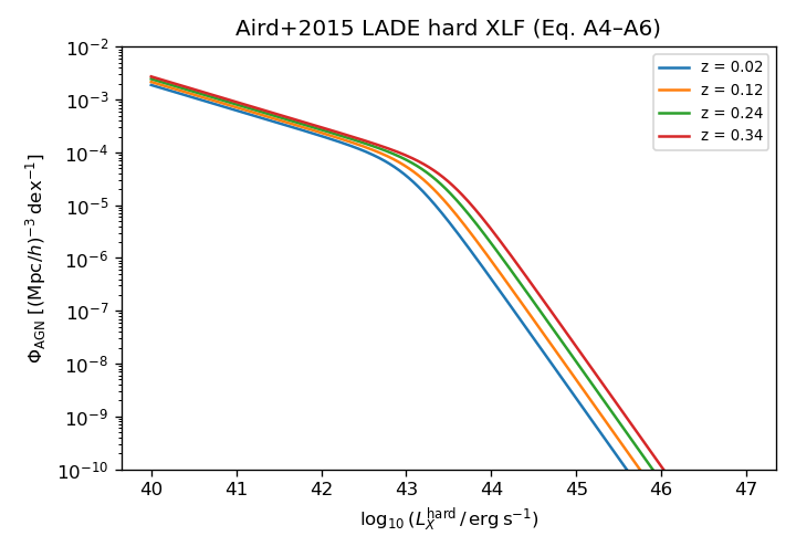
Hard-band XLF \(\Phi_\mathrm{AGN}(L_X,z)\) at several redshifts.
Step 2 — hard \(L_X\) \(\to\) observed soft flux
Each hard luminosity is mapped to an observed soft (0.5–2 keV) flux by going
through the same steps as the HAM AGN model: an obscuration distribution
(Comparat+2019) sets an obscuration-weighted K-correction
\(k_\mathrm{eff}(L_X,z)\) (XSPEC table,
mean_k_eff()), giving
\(S_X = 10^{\log_{10}L_X + \log_{10}k_\mathrm{eff}} / (4\pi d_L^2)\).
The cross-correlation is between the galaxies and all X-ray events, so no optical (r-band) selection is applied — every AGN whose k-corrected soft flux lies in the range \([10^{-20}, 10^{-10}]\,\mathrm{erg\,s^{-1}cm^{-2}}\) (Lau+2025) contributes. The flux completeness is taken as \(f(S_X)=1\) (unlike Lau et al. 2025, who use a logistic flux-limit curve, Eq. A11).
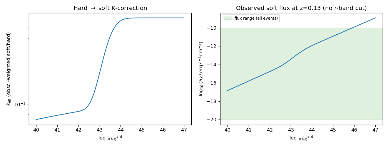
K-correction \(k_\mathrm{eff}\) and the observed soft flux \(S_X(L_X)\) at the sample mean redshift; no r-band cut is applied.
Step 3 — the \(W_\mathrm{AGN}(z)\) kernel (Eq. A9)
The X-ray-flux-weighted redshift kernel is
integrated over all AGN in the k-corrected flux range (no optical selection),
with the number density
\(n_\mathrm{AGN}(z) = \int \mathrm{d}\ln L_X\,\Phi_\mathrm{AGN}\,f\)
and the number-weighted mean flux
\(\langle S_X\rangle(z) = W_\mathrm{AGN}(z)/n_\mathrm{AGN}(z)\). This is
computed once per sample and stored, with all integrand components, to
results/agn_duty_cycle/W_AGN_<sample>.h5 (skipped if it exists):
python -m hod_mod.scripts.galaxies.precompute_w_agn --sample S1
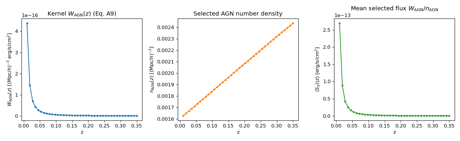
The kernel \(W_\mathrm{AGN}(z)\), the selected number density \(n_\mathrm{AGN}(z)\), and the mean selected flux \(\langle S_X\rangle(z)\) for S1.
Step 4 — occupation \(\times\) duty cycle
The AGN occupation is the fixed ZM15 occupation (centrals + satellites, Eqs. 21–22) scaled by a single duty cycle \(DC = 10^{\log_{10}DC}\) with the physical prior \(DC \in [0.001, 0.5]\) (i.e. \(\log_{10}DC \in [-3, -0.301]\); the AGN-host fraction is between 0.1 % and 50 %), times a high-mass cutoff \(C(M_h)\):
Because ZM15 satellites scale with the centrals, putting the duty cycle in front of the central occupation propagates to the satellites. The cutoff \(C(M_h)\) is a smooth cosine taper that is 1 below \(10^{14}\,M_\odot/h\) and declines to 0 at \(2\times10^{14}\,M_\odot/h\), so that X-ray AGN are not hosted by the most massive (cluster-scale) halos — both the central and satellite AGN occupation vanish above \(\log_{10}M_h \simeq 14.3\). This removes the cluster-scale AGN contribution from the cross-power (mainly the 1-halo satellite and two-halo terms on medium/large scales); the galaxy occupation itself is unchanged.
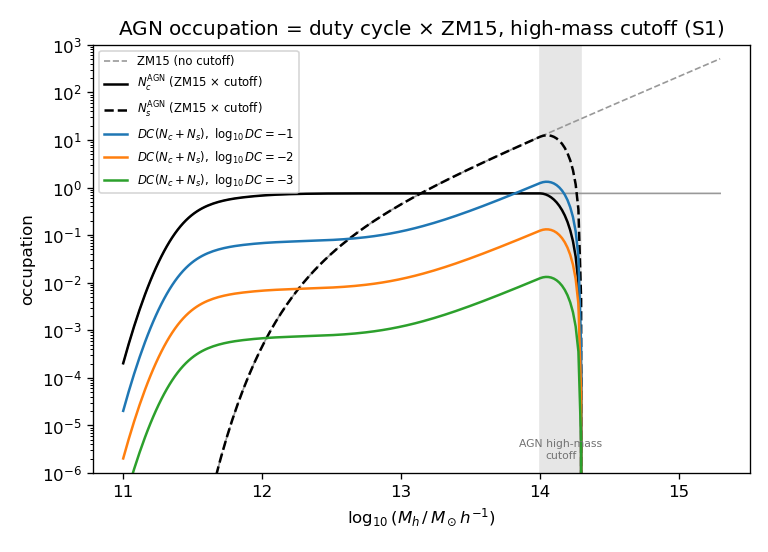
AGN occupation = ZM15 \(\times\) high-mass cutoff (× duty cycle). The grey curves are the raw ZM15 (no cutoff); the black/coloured curves drop to zero across the shaded band (\(10^{14}\)–\(2\times10^{14}\,M_\odot/h\)).
Step 5 — cross-power and \(w(\theta)\) (Eqs. A7/A8 for the cross)
The Lau et al. 2025 1-/2-halo AGN power spectra (Eqs. A7/A8) are modified for the galaxy \(\times\) AGN-emission cross-correlation by replacing the AGN auto-occupation with the product of the galaxy and AGN occupations, with \(u_\mathrm{AGN} = u_\mathrm{NFW}\). The per-AGN soft luminosity is mass-independent, \(\langle L_X\rangle(z) = \langle S_X\rangle(z)\, 4\pi d_L^2(z)\), so the cross-power is linear in the duty cycle:
with \(u_\mathrm{AGN}\) the NFW Fourier transform (Eq. A10). The cross is
realised through the existing
angular_cl_gX()
path (Limber + eROSITA King PSF, \(\theta_c = 8.64''\)), so the AGN and gas
contributions are summed in consistent internal units; \(w(\theta)\) follows
from the Hankel transform of \(C_\ell\).
The flux \(\to\) count conversion is computed, not fitted
The Comparat 2025 GALxEVT \(w(\theta)\) is a count ratio (the
Davis–Peebles estimator \(w = (S^G_X-S^R_X)/S^R_X\)), converted to a
physical surface brightness by multiplying by the background
\(S^R_X\) (beckground column, in
\(\mathrm{erg\,kpc^{-2}\,s^{-1}}\)). Rather than absorb the flux
\(\to\) count conversion into a free amplitude, we compute it from the
real eROSITA instrument: each component is folded through the true
energy-conversion factor (ECF) from the DR1 TM0 survey ARF + RMF
(ErositaResponse), tabulated band-averages over
0.5–2 keV for the gas (APEC at the halo temperature \(kT(M)\)) and the
AGN (absorbed power law \(\Gamma=1.9\)). The model \(\to\) data gas
normalisation \(C_\mathrm{total}\) (the amplitude the fiducial-density
gas produces) then follows from the cooling function \(\Lambda\), the
ECF, and \(S^R_X\) (\(C_\mathrm{total}\propto1/S^R_X\)), anchored once
on S1 where the fiducial DPM density reproduces the data. This removes the
free normalisation factors log10_A_gas and log10_A_AGN: the gas leg
is parametrised directly by the physical central density
\(\log_{10}n_{e,0.3}\) (\(A_\mathrm{gas}=C_\mathrm{total}\,
(n_e/n_e^\mathrm{fid})^2\)) and the AGN leg by the duty cycle
\(\log_{10}DC\) (\(A_\mathrm{AGN}=10^{\log_{10}DC+C_\mathrm{obs}}\)).
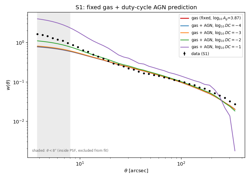
S1 prediction with the gas fixed at the data-validated fixed-ZM15 MAP (\(\log_{10}A_\mathrm{gas}=3.87\), \(\beta_\mathrm{gas}=0.25\), \(\beta_P=0.86\)) and the duty-cycle AGN added for \(\log_{10}DC = -4,-3,-2,-1\). \(\log_{10}DC=-2\) tracks the data; \(-1\) over-predicts the small-scale signal and \(-4,-3\) reduce to gas-only. The shaded band (\(\theta<8''\)) is inside the PSF and excluded from the fit.
Running the baseline MAP fit (physical parameters)
The baseline MAP fit (hod_mod.scripts.fitting.fit_agn_duty_cycle_baseline)
holds the ZM15 galaxy occupation fixed at the multi-mass-bin MAP and varies
the five physical parameters
\(\{\log_{10}n_{e,0.3}, \beta_\mathrm{gas}, p_2, r_\mathrm{max},
\log_{10}DC\}\) over \(\theta\in[8,300]''\). There are no free normalisation
factors: the gas amplitude is \(A_\mathrm{gas}=C_\mathrm{total}\,
(n_e/n_e^\mathrm{fid})^2\) with the computed conversion \(C_\mathrm{total}\),
and the AGN amplitude is \(A_\mathrm{AGN}=10^{\log_{10}DC+C_\mathrm{obs}}\).
The two linear amplitudes are still solved analytically (bounded least squares,
now bounded to the physical priors \(n_e/n_e^\mathrm{fid}\in[0.1,10]\)
and \(DC\in[0.001,0.5]\)), so the optimizer searches only the
\((\beta_\mathrm{gas}, p_2, r_\mathrm{max})\) shape:
JAX_PLATFORMS=cpu python -m hod_mod.scripts.fitting.fit_agn_duty_cycle_baseline \
    --sample S1 --map-only        # add --nsteps for the MCMC
Results are written to results/agn_duty_cycle/baseline/<sample>_baseline_map.json.
The same fixed ZM15 is used for every sample; only the stellar-mass threshold and
\(n(z)\) change.
Sample |
\(\log_{10}M_*^\mathrm{min}\) |
\(n_e/n_e^\mathrm{fid}\) |
\(\beta_\mathrm{gas}\) |
\(p_2\) |
\(\log_{10}DC\) |
\(DC\) |
\(\chi^2/\mathrm{dof}\) |
|---|---|---|---|---|---|---|---|
S1 |
10.00 |
10 (rail) |
1.63 |
0.60 |
−1.95 |
0.011 |
1.63 |
S3 |
10.50 |
1.5 |
1.60 |
1.20 |
−1.66 |
0.022 |
1.56 |
S5 |
11.00 |
10 (rail) |
0.40 |
2.40 |
−1.67 |
0.021 |
4.88 |
S7 |
11.50 |
10 (rail) |
1.60 |
0.78 |
−3.0 (rail) |
0.001 |
111.7 |
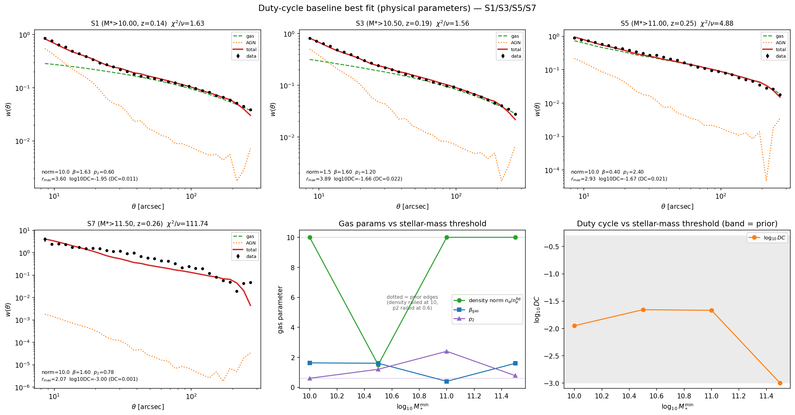
Best-fit \(w(\theta)\) decomposition (data, gas, AGN, total) for S1/S3/S5/S7 and the physical parameters vs stellar-mass threshold. The gas dominates; the density prior rails at \(10\times\) fiducial for S1/S5/S7 while S3 sits cleanly at \(1.5\times\); S7 under-predicts the data at \(\theta>30''\).
Open issue — the gas amplitude wants to run away at high mass
With physical density priors the fit is clean only for the low thresholds (S3 \(\chi^2/\mathrm{dof}=1.56\), \(n_e=1.5\, n_e^\mathrm{fid}\)). For the higher-mass samples the gas density rails at \(10\times\) fiducial and the fit degrades sharply (S5 \(4.9\), S7 \(112\)): the data require much more gas than 10× fiducial. Two effects contribute and define the way forward: (i) the model \(\to\) data conversion \(C_\mathrm{total}\) is anchored on S1 and transferred by \(1/S^R_X\) only — it must be calibrated per sample from each sample’s own fiducial-gas prediction (the galaxy density \(n_g\), bias and \(n(z)\) differ with the threshold); and (ii) the galaxy \(\times\) gas and galaxy \(\times\) AGN cross-powers are nearly degenerate in \(\theta\)-shape over \([8,300]''\), so breaking the degeneracy needs either the X-ray auto-power, the stacked surface-brightness profile, or an external gas-density prior (e.g. the \(L_X\)–\(M\) scaling relation).
BGS LS10 MAP results — samples S1–S3
Fitting script:
hod_mod.scripts.fitting.fit_comparat2025
(--mode map, --sample S1).
Data: BGS LS10 galaxy catalogue × eROSITA all-sky soft X-ray (0.5–2 keV)
+ BGS LS10 clustering \(w_p(r_p)\) from
Comparat et al. 2025 (arXiv:2503.19796).
Sample |
\(\log_{10} M_*^\mathrm{min}\) |
\(z_\mathrm{mean}\) |
\(N_\mathrm{gal}\) |
\(\chi^2/\mathrm{dof}\) |
npts (\(w_\theta\) + \(w_p\)) |
Status |
|---|---|---|---|---|---|---|
S1 |
10.00 |
0.135 |
2 759 238 |
3.85 |
57 (31 + 26) |
elevated |
S2 |
10.25 |
0.162 |
3 308 841 |
0.07 |
31 (\(w_\theta\) only) |
good |
S3 |
10.50 |
0.191 |
3 263 228 |
23.17 |
57 (31 + 26) |
poor fit |
Parameter |
S1 |
S2 |
S3 |
|---|---|---|---|
|
3.988 |
6.802 |
3.626 |
|
0.244 |
0.232 |
0.618 |
|
0.891 |
0.909 |
2.000 (at bound) |
|
0.086 |
0.132 |
0.364 |
|
9.546 |
10.234 |
9.000 (at bound) |
|
0.562 |
0.500 |
0.871 |
|
9.988 |
12.061 |
9.500 (at bound) |
|
0.924 |
1.054 |
0.822 |
Note
S1 column refreshed 2026-06-16 with the current code
(fit_comparat2025.py); the previous S1 entries here (\(\chi^2/\mathrm{dof}=23.00\),
log10_A_gas=7.760, log10_A_AGN=0.231) were generated before
same-day fixes to the gas/AGN cross-spectra code and are stale. S2 and S3
have not been refreshed and may likewise be out of date relative to the
current code.
Note
S1 (\(\chi^2/\mathrm{dof}=3.85\)) and S3 (\(\chi^2/\mathrm{dof}=23.17\), not yet refreshed) remain \(\gg 1\). The ZM15 iHOD model was calibrated on SDSS (\(z \approx 0.1\), small-scale \(r_p \gtrsim 0.05\,h^{-1}\,\mathrm{Mpc}\)). BGS LS10 spans higher redshifts and includes scales \(r_p < 0.1\,h^{-1}\,\mathrm{Mpc}\) where fibre-collision corrections and non-linear satellite dynamics may introduce systematic offsets. S2 (\(\chi^2/\mathrm{dof} = 0.07\)) is fitted with \(w_\theta\) only (no \(w_p\) data available for this sample), which accounts for the much lower \(\chi^2\).
S3 beta_pressure and lg_m1h reach their prior boundaries —
this sample requires wider priors or a different model.
AGN luminosity calibration check
log10_A_AGN is a free linear amplitude on a normalized PSF template
(_psf_template()), fit
directly against the dimensionless \(w(\theta)\) data. By construction it
has no built-in link to HamAGNModel’s
predicted mean soft X-ray AGN luminosity — so “log10_A_AGN close to 0”
is not, by itself, evidence that the model’s AGN luminosity is correct.
hod_mod.scripts.fitting.audit_agn_lx_comparat2025 builds that missing
link using the background-subtraction technique of Comparat et al. 2025
(\(S_X^G(R) = (1+w(R))\times S_R^X\), their Eq. 3 and Table 2): the
fitted AGN amplitude is converted into a physical excess surface-brightness
profile and integrated over area to give a mean AGN luminosity, which is then
compared to (a) HamAGNModel.mean_agn_lx() evaluated with the
central-galaxy-occupation-weighted halo population (matching the paper’s
“AGN only in centrals” assumption), and (b) Comparat+2025 Table 4’s
independently deduced point-source luminosity.
Quantity |
Value |
Notes |
|---|---|---|
\(L_X\) implied by the fit |
\(3.08\times10^{40}\) erg/s |
via \(A_\mathrm{AGN}\times\mathrm{PSF}(\theta)\times S_R^X\) |
\(L_X\) deduced, Comparat+2025 Table 4 |
\(3.59\times10^{40}\) erg/s |
independent measurement; ratio to fit-implied = 0.86 |
The fit-implied value agrees with the paper’s independently-deduced value to
14% — the background-subtraction conversion (
hod_mod.scripts.fitting.audit_agn_lx_comparat2025) is working
correctly. The background-value table used (Table 2) calibrates the
Davis-Peebles stacking estimator, while wtheta here is the Landy-Szalay
estimator — the paper shows these agree to ~5-10% over 20-500 kpc (proper)
and diverge outside that range, a systematic worth keeping in mind.
``HamAGNModel`` calibration against Table 4 (all 7 samples).
hod_mod.scripts.fitting.calibrate_ham_agn_lx fits 3 free parameters
added to mean_agn_log10lx — scatter_lx (overrides the constructor’s
scatter, cheap since it never touches the abundance-matching precompute),
log10_A_kcorr (rescales the K-correction, clamped ≤1), log10_A_dc
(rescales the duty cycle used in population-averaging only, not the one
baked into the abundance-matching table) — against Table 4, using
_TABLE3-default HOD parameters throughout (decoupled from any w(θ)
MAP-fit staleness).
Sample |
floor_fraction |
\(L_X\) raw [erg/s] |
\(L_X\) paper [erg/s] |
ratio |
|---|---|---|---|---|
S1 |
0.868 |
\(4.24\times10^{39}\) |
\(3.59\times10^{40}\) |
0.12 |
S2 |
0.000 |
\(2.77\times10^{41}\) |
\(4.54\times10^{40}\) |
6.10 |
S3 |
0.000 |
\(4.62\times10^{41}\) |
\(6.20\times10^{40}\) |
7.45 |
S4 |
0.000 |
\(8.69\times10^{41}\) |
\(8.63\times10^{40}\) |
10.06 |
S5 |
0.000 |
\(1.74\times10^{42}\) |
\(7.60\times10^{40}\) |
22.92 |
S6 |
0.000 |
\(3.46\times10^{42}\) |
\(7.43\times10^{40}\) |
46.58 |
S7 |
0.000 |
\(7.39\times10^{42}\) |
\(5.53\times10^{40}\) |
133.54 |
Two distinct, independent problems, not one:
S1 (only): floor-saturated, not a calibration target. 86.8% of S1’s HOD-\(N_\mathrm{cen}\)-weighted population sits at
HamAGNModel’s physical luminosity floor (_LOG10_LX_MIN_PHYSICAL = 40.0dex). This is not a numerical-resolution artifact: the Aird+2015 faint-end slope makes the abundance-matched luminosity diverge (verified directly, no convergence extending the grid down to 26 dex) for halos as low-mass as S1’s stellar-mass threshold (9.56, the lowest of the 7) pulls in. 40.0 dex was chosen as a physically-motivated minimum (roughly the conventional low-luminosity-AGN/XRB boundary), not derived from data, so S1’s prediction is dominated by that assumption and excluded from the fit below.S2–S7: a clean, monotonically growing over-prediction with stellar-mass threshold (6× at S2 up to 134× at S7) that 3 flat multiplicative parameters cannot absorb — confirmed by running the calibration:
Parameter |
Best fit |
|---|---|
|
0.550 dex (default 0.8) |
|
−0.197 |
|
−0.351 |
Sample |
\(L_X\) calibrated [erg/s] |
\(L_X\) paper [erg/s] |
ratio |
\(L_X\) fit-implied [erg/s] |
|---|---|---|---|---|
S1 |
\(4.90\times10^{38}\) |
\(3.59\times10^{40}\) |
0.01 |
\(3.08\times10^{40}\) |
S2 |
\(3.20\times10^{40}\) |
\(4.54\times10^{40}\) |
0.71 |
\(1.80\times10^{40}\) |
S3 |
\(5.34\times10^{40}\) |
\(6.20\times10^{40}\) |
0.86 |
\(5.26\times10^{40}\) |
S4 |
\(1.01\times10^{41}\) |
\(8.63\times10^{40}\) |
1.16 |
\(2.71\times10^{40}\) |
S5 |
\(2.02\times10^{41}\) |
\(7.60\times10^{40}\) |
2.65 |
n/a (stale) |
S6 |
\(4.00\times10^{41}\) |
\(7.43\times10^{40}\) |
5.39 |
\(1.82\times10^{41}\) |
S7 |
\(8.54\times10^{41}\) |
\(5.53\times10^{40}\) |
15.45 |
\(1.69\times10^{41}\) |
The calibration brings S2–S4 within ~30% of Table 4, but the residual
grows systematically with stellar-mass threshold for S5–S7 (2.7× to
15×) — none of the 3 fitted parameters is pinned at its bound, so this isn’t
“the optimizer wants to go further and can’t”; a flat amplitude genuinely
cannot reproduce a trend that grows over two decades in mass. The most
likely explanation: this codebase weights HamAGNModel by the full
galaxy-sample HOD occupation (_TABLE3, the same threshold used for
\(w_p(r_p)\) clustering), while Comparat+2025’s Table 4 values are
deduced using Comparat+2023’s AGN-specific HOD (a much higher effective
mass threshold than the full galaxy sample, with a free ΔM_min shift) —
i.e. the two are integrating over different halo populations, increasingly
so at the high-mass end. Adopting an AGN-specific threshold for this
weighting (rather than rescaling HamAGNModel’s amplitude further) is the
recommended next step; not implemented here. See
results/fits/comparat2025/ham_agn_calibration.json for full per-sample
detail and hod_mod.scripts.fitting.calibrate_ham_agn_lx.
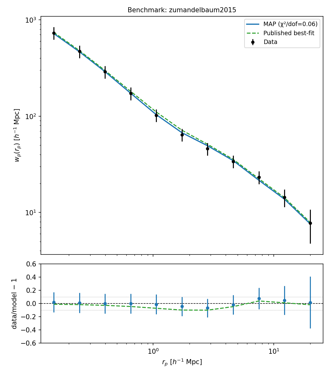
SDSS DR7 \(w_p(r_p)\) at MAP (ZM15 published parameters).
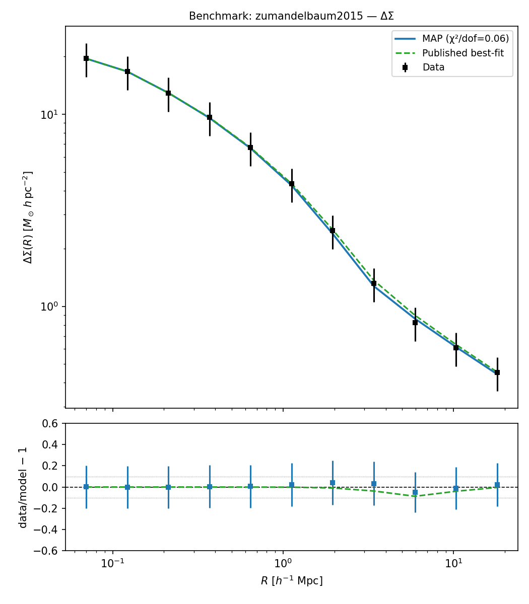
SDSS DR7 \(\Delta\Sigma(R)\) at MAP (ZM15 published parameters).
Timing — CPU vs GPU
The joint BGS fit (hod_mod.scripts.fitting.bgs_ls10.fit_bgs_zm15_joint)
runs on JAX, so it can execute on either CPU or GPU. The backend is selected
per process by the JAX_PLATFORMS environment variable (cpu or cuda);
the hod_mod environment sets JAX_PLATFORMS=cpu by default.
For this fit, CPU is faster — by roughly 4× per likelihood evaluation and ~2×
in JIT-compile time. The benchmark below times one
JointZM15.log_prob() evaluation (the fit’s compute core: for each of the 8
LS10-BGS stellar-mass bins it predicts \(w_p(r_p)\) via the Ogata
\(j_0\) Hankel transform plus \(\bar n_g\)), measured on an NVIDIA
RTX 3060 Laptop GPU vs CPU with jax 0.9.2 (wp + n_gal, no lensing).
Metric |
CPU |
GPU (RTX 3060) |
Winner |
|---|---|---|---|
Infra build (CAMB + HMF) |
0.22 s |
0.29 s |
~tie |
First call / JIT compile |
245 s |
477 s |
CPU ~2× |
Steady-state per evaluation |
8.5 s |
34.9 s (±6.1) |
CPU ~4.1× |
|
−20889.4994 |
−20889.4943 |
match (float tol) |
The matching log_prob values confirm an identical workload on both backends.
Why the GPU is slower here
This is the expected behaviour for this workload, not a misconfiguration:
The halo-model arrays are modest (\(n_k\approx1024\), \(n_m\approx512\)) and do not saturate the GPU.
The likelihood is a Python loop over the 8 mass bins, each performing an Ogata \(j_0\) Hankel transform — many small sequential kernels — and each
log_probreturns a scalar toscipy/emcee, forcing a host↔device synchronisation every call. GPU kernel-launch and transfer overhead therefore dominate (and drive the large ±6 s scatter).XLA’s GPU compilation is heavier (477 s vs 245 s).
Recommendation: run the fit on CPU (keep JAX_PLATFORMS=cpu). The GPU
gives no benefit here. At ~8.5 s/eval on CPU, a full Powell MAP or an
80,000-evaluation MCMC is expensive; the lever for speed is the per-evaluation
cost itself (e.g. coarser \(w_p\) \(k\)/\(r\) grids, or vectorising
the per-bin loop), not the GPU.
Reproducing the benchmark
The harness hod_mod.scripts.timing.bench_bgs_zm15_joint times
log_prob (separating JIT compile from steady state, with a host-device sync
each call for correct asynchronous-GPU timing):
# both backends + comparison table in one command
python -m hod_mod.scripts.timing.bench_bgs_zm15_joint --both

# single backend
JAX_PLATFORMS=cpu  python -m hod_mod.scripts.timing.bench_bgs_zm15_joint
JAX_PLATFORMS=cuda python -m hod_mod.scripts.timing.bench_bgs_zm15_joint

# include lensing (ESD) in the timed workload
python -m hod_mod.scripts.timing.bench_bgs_zm15_joint --both --surveys HSC DES KIDS
References and external resources
All links below were verified to resolve to the cited work. References that the code uses but for which a stable preprint link could not be verified are listed by author/year only (no link), to avoid mis-citation.
Methods and models (verified preprints)
Galaxy occupation (iHOD) — Zu & Mandelbaum 2015, arXiv:1505.02781 (“Mapping stellar content to dark matter halos … SDSS DR7”).
Halo mass function — Tinker et al. 2008, arXiv:0803.2706; halo bias — Tinker et al. 2010, arXiv:1001.3162.
Halo concentration — Diemer & Joyce 2019, arXiv:1809.07326.
Non-linear / beyond-linear bias (HMcode-2020) — Mead et al. 2021, arXiv:2009.01858.
Cosmological parameters — Planck 2018, arXiv:1807.06209.
Gas profiles (Descriptive Parametric Model, DPM) — arXiv:2505.14782.
Cluster pressure profile (A10 / REXCESS) — Arnaud et al. 2010, arXiv:0910.1234.
AGN X-ray luminosity function (LADE) — Aird et al. 2015, arXiv:1503.01120.
Galaxy × AGN/diffuse X-ray cross-power (Appendix A) — Lau et al. 2025, arXiv:2410.22397.
Galaxy × soft-X-ray cross-correlation (GALxEVT data + method) — Comparat et al. 2025, arXiv:2503.19796.
SRG/eROSITA telescope — Predehl et al. 2021, arXiv:2010.03477; eROSITA DR1 — Merloni et al. 2024, arXiv:2401.17274.
Data and software (verified)
eROSITA-DE DR1 — https://erosita.mpe.mpg.de/dr1/ ; instrument responses (ARF/RMF, TM0 survey + on-axis): https://erosita.mpe.mpg.de/dr1/eSASS4DR1/eSASS4DR1_arfrmf/ .
Legacy Surveys DR10 (LS10 galaxies) — https://www.legacysurvey.org/dr10/ .
GALxEVT cross-correlation measurements (data) — Zenodo record 15111974, https://doi.org/10.5281/zenodo.15111974 .
AtomDB / APEC plasma emission — https://hea-www.cfa.harvard.edu/AtomDB/ .
SOXS (X-ray response folding, ARF/RMF, ECF) — https://hea-www.cfa.harvard.edu/soxs/ .
Cited by name only (no verified preprint link)
X-ray scaling relations used to validate the gas (\(L_X\)–\(M\), \(kT\)–\(M\)) — Lovisari et al. 2020; Bulbul et al. 2018; Lovisari et al. 2015 (groups). (The arXiv identifier recorded in the code for Lovisari+2020 is incorrect and is not reproduced here.)