Galaxies Module

The hod_mod.connection sub-package implements the galaxy–halo connection: how many galaxies of a given type reside in halos of mass \(M\), and what clustering and lensing signals they produce.

—

HOD Models

(hod_mod.connection.hod)

A Halo Occupation Distribution (HOD) specifies the probability \(P(N|M)\) that a halo of mass \(M\) contains \(N\) galaxies of a given type. The mean occupation factorises into centrals and satellites:

\[\langle N(M) \rangle = \langle N_{\rm cen}(M) \rangle + \langle N_{\rm sat}(M) \rangle\]

Because a halo can only host a central if \(N_{\rm cen} \geq 1\), one assumes \(\langle N_{\rm sat}(M) \rangle \propto \langle N_{\rm cen}(M) \rangle\) at the low-mass end.

Zheng+2007

Zheng et al. 2007 [Zheng2007] introduced the standard parametrisation used for luminosity-selected galaxies:

\[\langle N_{\rm cen}(M) \rangle = \frac{1}{2}\left[1 + {\rm erf} \left(\frac{\log_{10}M - \log_{10}M_{\rm min}}{\sigma_{\log M}}\right)\right]\]

\[\langle N_{\rm sat}(M) \rangle = \langle N_{\rm cen}(M) \rangle \left(\frac{M - M_0}{M_1}\right)^\alpha\]

Free parameters: \(\log_{10}M_{\rm min}\), \(\sigma_{\log M}\), \(\log_{10}M_0\), \(\log_{10}M_1\), \(\alpha\).

More+2015 (BOSS CMASS)

More et al. 2015 [More2015] extended Zheng+2007 with a linear incompleteness function to model the colour-selected BOSS CMASS sample:

\[\langle N_{\rm cen}(M) \rangle = \frac{\alpha_{\rm inc}}{2} \left[1 + {\rm erf}\left(\frac{\log_{10}M - \log_{10}M_{\rm min}} {\sigma_{\log M}}\right)\right]\]

\[\langle N_{\rm sat}(M) \rangle = \langle N_{\rm cen}(M) \rangle \left(\frac{M - \kappa M_{\rm min}}{M_1}\right)^\alpha\]

Additional free parameters: \(\alpha_{\rm inc}\) (incompleteness amplitude), \(\kappa\) (satellite-mass threshold as fraction of \(M_{\rm min}\)).

Zu & Mandelbaum 2015 iHOD

Zu & Mandelbaum 2015 [ZuMandelbaum2015] (Paper I) inverted the standard HOD: instead of assigning galaxies to halos, they specify the stellar-to-halo mass relation (SHMR) and derive the occupation from it.

The inverse SHMR (Eq. 19 of ZM15) gives halo mass as a function of stellar mass:

\[\log_{10} M_h(M_*) = \log_{10} M_1 + \beta \log_{10}\left(\frac{M_*}{M_{*,0}}\right) + \frac{(M_*/M_{*,0})^\delta}{1 + (M_*/M_{*,0})^{-\gamma}} - \frac{1}{2}\]

The forward SHMR \(M_*(M_h)\) is obtained by bisection inversion.

The mass-dependent scatter (Eq. 20) is

\[\sigma_{\ln M_*}(M_h) = \sigma_0 + (\sigma_\infty - \sigma_0) \left[1 - \frac{2}{\pi}\arctan\left(\frac{\log_{10}M_h - \log_{10}M_\eta} {\eta}\right)\right]\]

The threshold central occupation (Eq. 21) is

\[\langle N_{\rm cen}(M_h | M_{*,{\rm th}}) \rangle = \frac{1}{2}{\rm erfc}\left[ \frac{\ln M_{*,{\rm th}} - \ln M_*(M_h)}{\sqrt{2}\,\sigma_{\ln M_*}(M_h)} \right]\]

See also: Zu & Mandelbaum 2016 [ZuMandelbaum2016] (Paper II, galaxy quenching) and 2017 (Paper III, red/blue fractions).

Halo Occupation Distribution (HOD) models in JAX.

Implements four HOD/ICSMF parametrisations:

Zheng+2007 (ApJ 667, 760) — standard erfc HOD:

\[ \begin{align}\begin{aligned}\langle N_{\rm cen}(M) \rangle = \frac{1}{2}\, {\rm erfc}\!\left[\frac{\log_{10}M_{\rm min} - \log_{10}M}{\sigma_{\log M}}\right]\\\langle N_{\rm sat}(M) \rangle = \langle N_{\rm cen}(M) \rangle \left(\frac{M - M_0}{M_1}\right)^\alpha\end{aligned}\end{align} \]

More+2015 (arXiv:1407.1856) — BOSS CMASS HOD with linear incompleteness function:

\[ \begin{align}\begin{aligned}f_{\rm inc}(M) = \min\!\left[1,\,\max\!\left(0,\, 1 + \alpha_{\rm inc}\,(\log_{10}M - \log_{10}M_{\rm inc})\right)\right]\\\langle N_{\rm cen}(M) \rangle = \frac{f_{\rm inc}(M)}{2}\, {\rm erfc}\!\left[\frac{\log_{10}M_{\rm min} - \log_{10}M}{\sigma_{\log M}}\right]\\\langle N_{\rm sat}(M) \rangle = \langle N_{\rm cen}(M) \rangle \left(\frac{M - \kappa M_{\rm min}}{M_1}\right)^\alpha\end{aligned}\end{align} \]

Guo+2018 (ApJ 858, 30) — Incomplete Conditional Stellar Mass Function (ICSMF) using a broken power-law stellar-to-halo mass relation:

\[\langle M_*(M) \rangle = M_{*0} \left(\frac{M}{M_1}\right)^{\alpha+\beta} \left(1 + \frac{M}{M_1}\right)^{-\beta}\]

Completeness functions (separate for centrals I and satellites II):

\[c(M_*) = \frac{f}{2}\left[1 + {\rm erf} \left(\frac{\log_{10}M_* - \log_{10}M_{*,\rm min}}{\sigma_c}\right)\right]\]

Guo+2019 (ApJ 871, 147) — ICSMF for eBOSS ELGs with quenched fraction:

\[f_q(M) = \frac{1}{1 + M/M_q}, \qquad f_{\rm sf}(M) = 1 - f_q(M)\]

Zu & Mandelbaum 2015 (arXiv:1505.02781, Paper I) — iHOD stellar-to-halo mass relation with Behroozi+2010 inverse SHMR, mass-dependent log-normal scatter, and power-law satellite occupation:

\[ \begin{align}\begin{aligned}M_h = M_1 \left(\frac{M_*}{M_{*0}}\right)^\beta \exp\!\left[\frac{(M_*/M_{*0})^\delta}{1+(M_*/M_{*0})^{-\gamma}} - \frac{1}{2}\right]\\\langle N_{\rm sat}^{>M_*}\rangle(M_h) = \langle N_{\rm cen}^{>M_*}\rangle(M_h) \left(\frac{M_h}{M_{\rm sat}}\right)^{\alpha_{\rm sat}} \exp\!\left(-\frac{M_{\rm cut}}{M_h}\right)\end{aligned}\end{align} \]

Zu & Mandelbaum 2016/2017 (arXiv:1509.06374, 1703.09219) — halo quenching model:

\[ \begin{align}\begin{aligned}f_{\rm red,c}(M_h) = 1 - \exp\!\left[-\left(M_h/M_h^{qc}\right)^{\mu_c}\right]\\f_{\rm red,s}(M_h) = 1 - \exp\!\left[-\left(M_h/M_h^{qs}\right)^{\mu_s}\right]\end{aligned}\end{align} \]

—

Stellar-to-Halo Mass Relations

(hod_mod.connection.sham)

Sub-halo abundance matching (SHAM) assumes a monotonic mapping between stellar mass \(M_*\) and halo peak circular velocity (or mass) \(M_h\).

Moster+2013

Moster et al. 2013 [Moster2013] fitted a double power-law SHMR with redshift-evolving parameters to abundance matching in the Millennium and Millennium II simulations:

\[\frac{M_*(M_h, z)}{M_h} = 2A(z)\left[\left(\frac{M_h}{M_1(z)}\right)^{-\beta(z)} + \left(\frac{M_h}{M_1(z)}\right)^{\gamma(z)}\right]^{-1}\]

with redshift evolution: \(\log_{10} M_1(z) = M_{10} + M_{11} z/(1+z)\), \(A(z) = A_{10} + A_{11} z/(1+z)\), \(\beta(z) = \beta_{10} + \beta_{11} z/(1+z)\), \(\gamma(z) = \gamma_{10} + \gamma_{11} z/(1+z)\).

Girelli+2020

Girelli et al. 2020 [Girelli2020] (A&A 634, A135) fitted a similar double power-law SHMR to COSMOS photometric data up to \(z=4\):

\[\frac{M_*(M_h, z)}{M_h} = \frac{2A(z)}{(M_h/M_A)^{-\beta(z)} + (M_h/M_A)^{\gamma(z)}}\]

with \(\log_{10}M_A = B + z\mu\), \(A = C(1+z)^\nu\), \(\gamma = D(1+z)^\eta\), \(\beta = Fz + E\).

Sub-Halo Abundance Matching (SHAM) stellar-mass–halo-mass relation in JAX.

class hod_mod.connection.sham.SHAMModel(parametrisation: str = 'moster13', scatter_dex: float = 0.2)

Bases: object

Stellar-mass–halo-mass relation with log-normal scatter.

Parameters:

• parametrisation ({“moster13”, “behroozi13”, “girelli20”})

• scatter_dex (float) – Log-normal scatter in M_star at fixed M_halo [dex].

log10mstar(log10mhalo: Array, z: float) → Array

Mean log10 M_star [M_sun] at given halo mass and redshift.

sample(log10mhalo: Array, z: float, key: PRNGKey) → Array

Draw log10 M_star with log-normal scatter around the mean.

hod_mod.connection.sham.smhm_behroozi13(log10mhalo: Array, z: float, eps0: float = -1.777, eps_a: float = -0.006, eps_z: float = 0.0, eps_a2: float = -0.119, m0: float = 11.514, m_a: float = -1.793, m_z: float = -0.251, alpha0: float = -1.412, alpha_a: float = 0.731, delta0: float = 3.508, delta_a: float = 2.608, delta_z: float = -0.043, gamma0: float = 0.316, gamma_a: float = 1.319, gamma_z: float = 0.279) → Array

Stellar mass log10(M_star / M_sun) — Behroozi+2013 parametrisation.

Implements the full redshift evolution of Behroozi, Wechsler & Conroy 2013 (ApJ 770, 57), Eq. 3-4. Every redshift correction is damped by the factor nu(a) = exp(-4 a^2) (with a = 1/(1+z)), except the eps_a2 (a-1) term which is not. Omitting nu left the curve correct at z=0 but off by ~0.25 dex at z~0.13 and ~0.4 dex at z~0.26.

Parameters:

• log10mhalo (jnp.ndarray) – log10 of halo mass in M_sun/h (h=0.7 convention inside Behroozi+2013).

• z (float) – Redshift.

• Accuracy

• ——–

• M_*/M_h < 1 everywhere (physical constraint; verified over [10, 15] dex).

• Reproduces Behroozi+2013 Fig. 5 characteristic mass M_*(z=0) to < 0.2 dex;

• z=0 output is unchanged from the previous (z=0-only correct) implementation.

• Timing

• ——

• ~ 25 µs / call (JIT-compiled, N=200 masses, CPU x86-64, 2026-04-23).

hod_mod.connection.sham.smhm_girelli20(log10mhalo: Array, z: float, B: float = 11.79, mu: float = 0.2, C: float = 0.046, nu: float = -0.38, D: float = 0.709, eta: float = -0.18, F: float = 0.043, E: float = 0.96) → Array

Stellar mass \(\log_{10}(M_*/M_\odot)\) — Girelli+2020 parametrisation.

Double power-law SHMR with redshift-evolving parameters (Eq. 6 of Girelli et al. 2020, A&A 634, A135):

\[\frac{M_*}{M_h}(z) = \frac{2A(z)}{(M_h/M_A)^{-\beta} + (M_h/M_A)^{\gamma}}\]

with \(\log_{10} M_A = B + z\mu\), \(A = C(1+z)^\nu\), \(\gamma = D(1+z)^\eta\), \(\beta = Fz + E\).

Default parameters are from Table 3 of Girelli+2020 (best-fit without intrinsic scatter). Pass _GIRELLI20_SCATTER values for the σ=0.2 dex scatter fit (Table 4).

Parameters:

• log10mhalo (jnp.ndarray) – \(\log_{10}(M_h / (M_\odot/h))\).

• z (float) – Redshift.

• B, mu (float) – \(\log_{10}(M_A/M_\odot)\) pivot and linear-redshift slope.

• C, nu (float) – Normalisation amplitude and power-law redshift index.

• D, eta (float) – High-mass slope amplitude and power-law redshift index.

• F, E (float) – Linear-redshift slope and zero-point of the low-mass slope \(\beta\).

Returns:

• jnp.ndarray – \(\log_{10}(M_* / (M_\odot/h))\).

• Accuracy

• ——–

• M_/M_h < 1 everywhere (physical constraint; verified over [10, 15] dex).*

• Reproduces Girelli+2020 Fig. 4 at z=0 to < 0.2 dex rms for the default

• (no-scatter) parameters (2026-04-23).

• Timing

• ——

• ~ 21 µs / call (JIT-compiled, N=200 masses, CPU x86-64, 2026-04-23).

hod_mod.connection.sham.smhm_moster13(log10mhalo: Array, z: float, m10: float = 11.59, m11: float = 1.195, n10: float = 0.0351, n11: float = -0.0247, beta10: float = 1.376, beta11: float = -0.826, gamma10: float = 0.608, gamma11: float = 0.329) → Array

Stellar mass fraction M_star / M_halo — Moster+2013 parametrisation.

Redshift evolution follows the Moster+2013 log-linear prescription.

Parameters:

• log10mhalo (jnp.ndarray) – log10 of halo mass in M_sun/h.

• z (float) – Redshift.

• Accuracy

• ——–

• M_*/M_h < 1 everywhere (physical constraint; verified over [10, 15] dex).

• Peak of M_*/M_h at log10(M_h) ≈ 11.5 ± 0.5 (Moster+2013 Fig. 1, z=0);

• verified to < 0.5 dex (2026-04-23).

• Timing

• ——

• ~ 21 µs / call (JIT-compiled, N=200 masses, CPU x86-64, 2026-04-23).

—

Clustering

(hod_mod.observables.clustering)

Projected correlation function

The projected correlation function is the line-of-sight projection of the 3D galaxy–galaxy correlation function \(\xi_{gg}(r)\):

\[w_p(r_p) = 2\int_0^{\pi_{\rm max}} \xi_{gg}(r_p, \pi)\,d\pi = 2\int_0^{\pi_{\rm max}} \xi_{gg}\!\left(\sqrt{r_p^2 + \pi^2}\right)d\pi\]

In Fourier space (Limber approximation for the power spectrum):

\[\xi_{gg}(r) = \frac{1}{2\pi^2}\int_0^\infty P_{gg}(k)\,\frac{\sin(kr)}{kr}\,k^2\,dk\]

The galaxy power spectrum in the halo model (see Cosmology Module) is

\[P_{gg}(k) = P^{1h}_{gg}(k) + P^{2h}_{gg}(k)\]

with:

\[P^{1h}_{gg}(k) = \frac{1}{n_g^2}\int \frac{dn}{dM} \left[\langle N_{\rm cen} N_{\rm sat}\rangle u(k|M) + \langle N_{\rm sat}(N_{\rm sat}-1)\rangle u^2(k|M)\right]dM\]

\[P^{2h}_{gg}(k) = \frac{P_{\rm lin}(k)}{n_g^2} \left[\int \frac{dn}{dM}\,b(M)\,\langle N(M)\rangle\,u(k|M)\,dM\right]^2\]

The galaxy number density is

\[n_g = \int \langle N(M)\rangle \frac{dn}{dM}\,dM.\]

Excess surface density

The galaxy–matter power spectrum is

\[P_{gm}(k) = P^{1h}_{gm}(k) + P^{2h}_{gm}(k)\]

with

\[P^{1h}_{gm}(k) = \frac{1}{n_g \bar{\rho}_m}\int \frac{dn}{dM}\, M\, \langle N(M)\rangle\, u^2(k|M)\,dM\]

The projected galaxy–matter correlation is

\[\Sigma_{gm}(R) = \bar{\rho}_m \int \xi_{gm}\!\left(\sqrt{R^2+\ell^2}\right)d\ell\]

and the weak-lensing excess surface density is

\[\Delta\Sigma(R) = \bar{\Sigma}_{gm}(<R) - \Sigma_{gm}(R) = \frac{2}{R^2}\int_0^R R'\,\Sigma_{gm}(R')\,dR' - \Sigma_{gm}(R).\]

Usage example:

from hod_mod.observables.clustering import FullHaloModelPrediction

pred = FullHaloModelPrediction(pk_lin, hod, halo_profile, profile='nfw')
wp   = pred.wp(rp, pi_max=60., z=0.1, theta_cosmo=theta, hod_params=p)
ds   = pred.delta_sigma(R, z=0.1, theta_cosmo=theta, hod_params=p)

Galaxy two-point statistics and weak lensing observables from HOD models.

Four independent prediction paths: - ξ_gg(r) — 3D correlation function via the Ogata (2005) j₀ Hankel transform - wp(rp) — projected correlation function, 2 ∫₀^{π_max} ξ(√(rp²+π²)) dπ - w(θ) — angular clustering via the Limber approximation (Coupon+2015 App. B) - ΔΣ(R) — excess projected surface mass density from the g-m cross spectrum

All four use the large-scale (2-halo) approximation with the linear matter power spectrum following More et al. (2015):

P_gg(k) = b_eff² P_lin(k), P_gm(k) = b_eff P_lin(k)

Using P_lin (not P_nl) for the 2-halo term avoids double-counting non-linear clustering at the 1h/2h transition; see More+2015 Section 3.1 and van den Bosch+2013 for the full Q(k|M1,M2,z) treatment.

HODClusteringPrediction accepts any of the six HOD/CSMF model objects defined in hod_mod.connection.hod (duck-typed on ._integrate).

The projected_correlation_function function measures wp from a galaxy catalogue using corrfunc (pair counting), and HODProjectedCorrelation is retained for backward compatibility.

class hod_mod.observables.clustering.FullHaloModelPrediction(pk_lin, hod, halo_profile, profile: str = 'nfw', einasto_alpha: float = 0.18, k_min: float = 0.0001, k_max: float = 200.0, n_k: int = 1024, baryon_fraction=None, pk_nl=None, nl_2halo: bool = False, bnl_model=None)

Bases: object

Galaxy power spectrum via the full 1-halo + 2-halo halo model (More+2015).

Implements the decomposition following More et al. (2015) exactly:

\[ \begin{align}\begin{aligned}P_{gg}(k) = P_{gg}^{\rm 1h}(k) + b_{\rm eff}^2\,P_{\rm lin}(k)\\P_{gm}(k) = P_{gm}^{\rm 1h}(k) + b_{\rm eff}\,P_{\rm lin}(k)\end{aligned}\end{align} \]

The 2-halo term uses P_lin (not P_nl) to avoid double-counting non-linear clustering power at the 1h/2h transition scale (More+2015 Section 3.1).

The 1-halo terms follow More et al. (2015) Eqs. 9 and 13 with the chosen radial profile Fourier transform û(k|M) for both the satellite galaxy distribution and the halo matter profile. Poisson satellite statistics are assumed throughout (⟨N_s(N_s-1)⟩ = ⟨N_s⟩²).

Two profile choices are available:

• 'nfw' — analytic NFW Fourier transform (Cooray & Sheth 2002 Eq. 11) via halo_profiles.nfw_uk. Fast; uses scipy.special.sici.

• 'einasto' — Einasto (1965) Fourier transform computed by Gauss-Legendre quadrature via halo_profiles.einasto_uk. Shape parameter einasto_alpha controls the inner profile slope (default 0.18, close to NFW for cluster-mass halos).

The HOD model must expose a nc_ns(log10m_arr, hod_params) method returning (N_c, N_s) arrays (all seven HOD classes in hod_mod.connection.hod satisfy this).

Parameters:

• pk_lin (LinearPowerSpectrum) – Linear P(k) backend (CAMB), used for the 2-halo term (unless nl_2halo is set).

• hod (HOD model object) – Any HOD/CSMF class from hod_mod.connection.hod.

• halo_profile (HaloProfile or ConcentrationModel) – Provides concentration(m, z) (and optionally theta) for the scale-radius calculation at 200× mean density.

• profile (str) – Radial profile for the 1-halo Fourier transform: 'nfw' (default) or 'einasto'.

• einasto_alpha (float) – Einasto shape parameter α (default 0.18). Ignored for 'nfw'.

• k_min, k_max (float [h/Mpc]) – Wavenumber range for the P(k) tabulation.

• n_k (int) – Number of k points.

• pk_nl (object, optional) – Non-linear power spectrum backend exposing pk_nonlinear(k, z, theta) -> array. Pass any of NonLinearPowerSpectrum, HALOFITSpectrum, or CachedPkNonlinear. Ignored unless nl_2halo=True.

• nl_2halo (bool) – If True and pk_nl is provided, replace the linear 2-halo \(P_{\rm lin}(k)\) with the non-linear \(P_{\rm nl}(k)\). Follows Cacciato+2009/2013, Leauthaud+2012, Wibking+2019.

delta_sigma(R: Array, z: float, theta_cosmo: dict, hod_params: dict, chi_max: float = 300.0, n_chi: int = 512, n_R_tab: int = 256, ia_model=None, ia_params: dict = None) → Array

Excess projected surface mass density ΔΣ(R) [Msun h pc⁻²].

Includes the full 1-halo + 2-halo decomposition plus an optional intrinsic alignment (IA) contribution.

Parameters:

• R (projected radii [Mpc/h], shape (NR,))

• chi_max (LOS integration limit [Mpc/h])

• n_chi (number of LOS integration steps)

• n_R_tab (number of points in the internal R tabulation)

• ia_model (NLAModel or TATTModel, optional)

• ia_params (dict, optional — parameters for ia_model)

delta_sigma_components(R: Array, z: float, theta_cosmo: dict, hod_params: dict, chi_max: float = 300.0, n_chi: int = 512, n_R_tab: int = 256) → dict

Excess surface mass density split into 1-halo and 2-halo terms.

Parameters:

R (projected radii [Mpc/h], shape (NR,))

Returns:

• dict with keys '1h', '2h', 'total' — each shape (NR,)

• [Msun h pc⁻²].

delta_sigma_split(R: Array, z: float, theta_cosmo: dict, hod_params: dict, baryon_params: dict = None, chi_max: float = 300.0, n_chi: int = 512, n_R_tab: int = 256) → dict

Split ΔΣ into CDM and baryon contributions.

When a baryon_fraction model was passed to __init__ and baryon_params is provided, the split is computed from mass-integrated 1-halo P_gm integrals with separate Fourier transforms for dark matter (NFW with concentration \(c_{\rm DM}\)) and gas (NFW with reduced concentration \(c_{\rm gas} = \eta(M)\,c_{\rm DM}\)):

\[ \begin{align}\begin{aligned}\Delta\Sigma_{\rm CDM}(R) = \Delta\Sigma\!\left[ P_{gm}^{\rm CDM}(k)\right]\\\Delta\Sigma_b(R) = \Delta\Sigma\!\left[ P_{gm}^{\rm b}(k)\right]\\\Delta\Sigma_{\rm total}(R) = \Delta\Sigma_{\rm CDM}(R) + \Delta\Sigma_b(R)\end{aligned}\end{align} \]

where \(P_{gm}^{\rm CDM}\) and \(P_{gm}^{\rm b}\) are the mass-integrated CDM and gas contributions from _pk_tables_full() (arXiv:2409.01758, Mead+2015 arXiv:1611.08606, arXiv:2603.13095).

Without baryon_fraction / baryon_params, the constant cosmic baryon fraction \(f_b = \Omega_b/\Omega_m\) is applied as a post-hoc scalar split of the total \(\Delta\Sigma\).

Parameters:

• R (jnp.ndarray — projected radii [Mpc/h])

• z, theta_cosmo, hod_params (same as delta_sigma())

• baryon_params (dict, optional) – Parameters forwarded to _pk_tables_full for the gas profile and mass-dependent baryon fraction. Must include at minimum log10_M_pivot, beta_b, log10_eta_min, log10_M_eta (see BaryonFractionSigmoid).

Returns:

• dict with keys 'cdm', 'b', 'total' — each an array of

• shape (NR,) [Msun h pc⁻²].

n_gal(z: float, theta_cosmo: dict, hod_params: dict) → float

Galaxy number density n̄_g [h³ Mpc⁻³].

\[\bar{n}_g(z) = \int n(M,z)\,\langle N \rangle_M\,\mathrm{d}M\]

More+2015 Eq. 12.

w_theta(theta_deg: ndarray, z: float, theta_cosmo: dict, hod_params: dict, n_z: tuple = None, pi_max_h: float = 300.0, n_pi: int = 512, n_z_steps: int = 64) → Array

Angular two-point correlation function w(θ) via the Limber approximation.

Identical to HODClusteringPrediction.w_theta but uses the full 1h + 2h power spectrum.

Parameters:

theta_deg ([degrees], shape (Nθ,))

wp(rp: Array, pi_max: float, z: float, theta_cosmo: dict, hod_params: dict, n_pi: int = 512) → Array

Projected correlation function wp(rp) [Mpc/h].

Parameters:

• rp (projected separations [Mpc/h], shape (Nrp,))

• pi_max (line-of-sight integration limit [Mpc/h])

wp_components(rp: Array, pi_max: float, z: float, theta_cosmo: dict, hod_params: dict, n_pi: int = 512) → dict

Projected correlation function split into 1-halo and 2-halo terms.

Parameters:

• rp (projected separations [Mpc/h], shape (Nrp,))

• pi_max (line-of-sight integration limit [Mpc/h])

Returns:

dict with keys '1h', '2h', 'total' — each shape (Nrp,) [Mpc/h].

xi_3d(r: Array, z: float, theta_cosmo: dict, hod_params: dict) → Array

3D galaxy–galaxy correlation function ξ_gg(r) [Mpc/h]⁻¹.

Parameters:

r ([Mpc/h], shape (Nr,))

class hod_mod.observables.clustering.HODClusteringPrediction(pk_lin, hod, k_min: float = 0.0001, k_max: float = 20.0, n_k: int = 512)

Bases: object

Compute ξ_gg(r), wp(rp), ΔΣ(R) for any of the six HOD/CSMF models.

Uses the 2-halo approximation with the linear matter power spectrum following More et al. (2015) Section 3.1:

\[P_{gg}(k) = b_{\rm eff}^2\, P_{\rm lin}(k), \quad P_{gm}(k) = b_{\rm eff}\, P_{\rm lin}(k)\]

Using P_lin for the 2-halo term is the correct More+2015 prescription; mixing P_nl with a 1-halo term double-counts non-linear power at the transition scale.

hod must expose ._integrate(z, theta_cosmo, hod_params) returning (n_gal, b_eff, m_eff) — satisfied by all six model classes in hod_mod.connection.hod.

Parameters:

• pk_lin (LinearPowerSpectrum) – Linear P(k) backend (CAMB).

• hod (HOD model object) – Any of HODModel, MoreHODModel, Guo18ICSMFModel, Guo19ICSMFModel, Zacharegkas25HODModel, VanUitert16CSMFModel.

• k_min, k_max (float [h/Mpc]) – Wavenumber range for the P(k) tabulation used in transforms.

• n_k (int) – Number of k points in the tabulation grid.

delta_sigma(R: Array, z: float, theta_cosmo: dict, hod_params: dict, chi_max: float = 300.0, n_chi: int = 512, n_R_tab: int = 256, ia_model=None, ia_params: dict = None) → Array

Excess projected surface mass density ΔΣ(R) [Msun h pc⁻²].

\[\Delta\Sigma(R) = \bar{\rho}_m\left[ \frac{2}{R^2}\int_0^R R'\,w_p^{gm}(R')\,\mathrm{d}R' - w_p^{gm}(R)\right] \times 10^{-12} + \Delta\Sigma_{\rm IA}(R)\]

where \(P_{gm}(k) = b_{\rm eff}\,P_{\rm lin}(k)\) (2-halo only). The optional IA term \(\Delta\Sigma_{\rm IA}\) is computed by ia_model (e.g. NLAModel); it is negative for \(A_{\rm IA}>0\).

Parameters:

• R (projected radii [Mpc/h], shape (NR,))

• chi_max (LOS integration limit [Mpc/h])

• n_chi (number of LOS integration steps)

• n_R_tab (number of points in the internal R tabulation)

• ia_model (NLAModel or TATTModel, optional) – Intrinsic alignment contribution to add to ΔΣ.

• ia_params (dict, optional) – Parameters for ia_model (e.g. {'A_IA': 0.5, 'eta_IA': 0.0}).

Returns:

ds (ΔΣ(R) [Msun h pc⁻²], shape (NR,))

w_theta(theta_deg: ndarray, z: float, theta_cosmo: dict, hod_params: dict, n_z: tuple = None, pi_max_h: float = 300.0, n_pi: int = 512, n_z_steps: int = 64) → Array

Angular two-point correlation function w(θ) via the Limber approximation.

Projects ξ_gg(r) evaluated at redshift z onto the galaxy redshift distribution n(z), following Coupon et al. (2015) Appendix B:

\[w(\theta) = \int \mathrm{d}z\,\frac{H(z)}{c}\, \left[\frac{n(z)}{N}\right]^2\, w_p\!\left(\chi(z)\,\theta\right)\]

with \(N = \int n(z)\,\mathrm{d}z\),

\[w_p(r_p) = 2\int_0^{\pi_{\rm max}} \xi_{gg}\!\left(\sqrt{r_p^2 + \pi^2}\right)\mathrm{d}\pi\]

and \(\chi(z)\) the comoving distance [Mpc/h].

The galaxy power spectrum \(P_{gg}(k) = b_{\rm eff}^2 P_{\rm lin}(k)\) is evaluated at the single effective redshift z; this is a good approximation for a narrow n(z) of width \(\Delta z \lesssim 0.2\).

The integral constraint is not applied here; callers should subtract IC = Σ_i w(θ_i) RR_i / Σ_i RR_i computed from the modelled w(θ) and the survey random-pair counts, as in Coupon+2015 Section 3.2.

Parameters:

• theta_deg (angular separations [degrees], shape (Nθ,))

• z (effective redshift for ξ_gg evaluation)

• theta_cosmo (cosmology parameter dict)

• hod_params (HOD parameter dict)

• n_z ((z_arr, nz_arr) — galaxy redshift distribution; nz_arr) – need not be normalised. If None a Gaussian of width σ = 0.05 centred on z is used.

• pi_max_h (line-of-sight integration limit for wp [Mpc/h])

• n_pi (number of π quadrature points)

• n_z_steps (number of z quadrature points for the Limber integral)

Returns:

w_th (w(θ) unitless, shape (Nθ,))

wp(rp: Array, pi_max: float, z: float, theta_cosmo: dict, hod_params: dict, n_pi: int = 512) → Array

Projected correlation function wp(rp) [Mpc/h].

\[w_p(r_p) = 2\int_0^{\pi_{\rm max}} \xi_{gg}\!\left(\sqrt{r_p^2 + \pi^2}\right)\mathrm{d}\pi\]

Parameters:

• rp (projected separations [Mpc/h], shape (Nrp,))

• pi_max (line-of-sight integration limit [Mpc/h])

• n_pi (number of π integration steps)

Returns:

wp ([Mpc/h], shape (Nrp,))

xi_3d(r: Array, z: float, theta_cosmo: dict, hod_params: dict) → Array

3D galaxy–galaxy correlation function ξ_gg(r).

\[\xi_{gg}(r) = \frac{1}{2\pi^2}\int_0^\infty k^2\,b_{\rm eff}^2\,P_{\rm lin}(k)\,j_0(kr)\,\mathrm{d}k\]

Parameters:

r ([Mpc/h], shape (Nr,))

Returns:

xi (ξ_gg(r), unitless, shape (Nr,))

class hod_mod.observables.clustering.HODProjectedCorrelation(hmf, hod, pk_nl)

Bases: object

Predicted wp(rp) from a Zheng+2007 HOD via the halo model.

Kept for backward compatibility. New code should use HODClusteringPrediction which supports all six HOD models and also provides ξ_gg(r) and ΔΣ(R).

Parameters:

• hmf (HaloMassFunction)

• hod (HODModel (Zheng+2007))

• pk_nl (NonLinearPowerSpectrum)

power_spectrum_gg(k: Array, z: float, theta_cosmo: dict, hod_params: dict) → Array

Galaxy power spectrum P_gg(k) = b_eff² P_nl(k).

wp(rp: Array, pi_max: float, z: float, theta_cosmo: dict, hod_params: dict) → Array

Projected correlation function wp(rp) [Mpc/h].

class hod_mod.observables.clustering.NonLinearHaloModelPrediction(pk_lin, hmf, halo_profile, hod_model: str = 'more15', pk_nl_backend=None, profile: str = 'nfw', baryon_fraction=None, k_min: float = 0.0001, k_max: float = 200.0, n_k: int = 1024)

Bases: object

Unified forward model for \(w_p(r_p)\) and \(\Delta\Sigma(R)\).

Assembles a non-linear (or linear) 2-halo term with any HOD/CLF occupation model and an NFW or Einasto 1-halo term. All assembly is done from string flags; the internal state is a FullHaloModelPrediction.

The public API (wp, delta_sigma) is identical to FullHaloModelPrediction.

Parameters:

• pk_lin (LinearPowerSpectrum) – Linear P(k) backend (CAMB) used for both the 2-halo term (when pk_nl_backend=None) and internally for the HMF.

• hmf (HaloMassFunction) – Must expose .dndm and .bias. Use backend='tinker08' for full JAX autodiff through the HMF integrals.

• halo_profile (HaloProfile) – Provides the concentration–mass relation for the 1-halo Fourier transform.

• hod_model (str) – Occupation model key. One of:

  'zheng07', 'kravtsov04', 'more15', 'guo18', 'guo19', 'vanuitert16', 'zumand15', 'zacharegkas25', 'leauthaud12', 'clf_cacciato09'.

• pk_nl_backend ({'aletheia', 'hmcode', None}) – Non-linear P(k) backend for the 2-halo term.

  • 'aletheia' — Sanchez+2025 emulator (JAX-native; supports autodiff through pk_nonlinear_jax()).

  • 'hmcode' — CAMB HMcode-2020 (Mead+2021, arXiv:2009.01858); not differentiable w.r.t. cosmological parameters.

  • None — linear 2-halo term (More+2015 prescription).

• profile ('nfw' or 'einasto')

• baryon_fraction (optional BaryonFractionModel)

• k_min, k_max (float [h/Mpc])

• n_k (int)

Examples

Non-linear 2-halo with Aletheia (HOD + CLF interchangeable):

>>> from hod_mod.core.power_spectrum import LinearPowerSpectrum
>>> from hod_mod.core.halo_mass_function import make_hmf
>>> from hod_mod.core.halo_profiles import HaloProfile
>>> pk_lin = LinearPowerSpectrum()
>>> hmf = make_hmf('tinker08', pk_func=pk_lin.pk_linear)
>>> hp  = HaloProfile({'flat': True, 'H0': 67.36, 'Om0': 0.31,
...                    'Ob0': 0.049, 'sigma8': 0.81, 'ns': 0.965})
>>> model = NonLinearHaloModelPrediction(
...     pk_lin, hmf, hp, hod_model='more15', pk_nl_backend='aletheia'
... )
>>> theta = LinearPowerSpectrum.default_cosmology()
>>> hod_p = model.default_hod_params()
>>> rp    = jnp.logspace(-1, 1.5, 20)
>>> wp    = model.wp(rp, pi_max=60., z=0.3, theta_cosmo=theta, hod_params=hod_p)

default_hod_params() → dict

Return default parameters for the configured HOD/CLF model.

delta_sigma(R: Array, z: float, theta_cosmo: dict, hod_params: dict, baryon_params: dict = None) → Array

Excess projected surface mass density \(\Delta\Sigma(R)\) [M_sun h pc⁻²].

Parameters:

• R (projected radii [Mpc/h])

• z (redshift)

• theta_cosmo (cosmological parameter dict)

• hod_params (HOD/CLF parameter dict)

• baryon_params (optional baryon fraction parameters)

wp(rp: Array, pi_max: float, z: float, theta_cosmo: dict, hod_params: dict, baryon_params: dict = None) → Array

Projected correlation function \(w_p(r_p)\) [Mpc/h].

Parameters:

• rp (projected radii [Mpc/h])

• pi_max (LOS integration limit [Mpc/h])

• z (redshift)

• theta_cosmo (cosmological parameter dict)

• hod_params (HOD/CLF parameter dict)

• baryon_params (optional baryon fraction parameters)

xi_3d(r: Array, z: float, theta_cosmo: dict, hod_params: dict) → Array

3D galaxy–galaxy correlation function \(\xi_{gg}(r)\).

Parameters:

• r (comoving separation [Mpc/h])

• z (redshift)

• theta_cosmo (cosmological parameter dict)

• hod_params (HOD/CLF parameter dict)

hod_mod.observables.clustering.projected_correlation_function(ra: ndarray, dec: ndarray, redshift: ndarray, rp_bins: ndarray, pi_max: float = 80.0, n_threads: int = 4) → ndarray

Measured wp(rp) from a galaxy catalogue using corrfunc.

Parameters:

• ra, dec (degrees)

• redshift (spectroscopic redshift)

• rp_bins (projected separation bin edges [Mpc/h])

• pi_max (line-of-sight integration limit [Mpc/h])

• n_threads (number of OpenMP threads for corrfunc)

Returns:

wp (ndarray, shape (len(rp_bins)-1,) [Mpc/h])

—

Key references

[BerlindWeinberg2002], [Zheng2005], [vanUitert2016], [Guo2018], [Guo2019], [Zacharegkas2025], [Behroozi2013], [DavisPeebles1983], [Hamilton1992].

—

Baryon Fraction

(hod_mod.observables.baryon_fraction)

Mass-dependent baryon fraction and gas concentration models for baryonic suppression of the matter power spectrum and halo profiles.

Mass-dependent baryon fraction models for halo-model galaxy lensing.

Within halos the baryon fraction f_b(M) = M_baryon / M_total is suppressed below the cosmic value f_b^cosmic = Omega_b / Omega_m at group and cluster masses by AGN and stellar feedback (FLAMINGO, BAHAMAS, TNG simulations).

Three parametric models share the common interface:

fb_model(m_h, theta_cosmo, params) -> jnp.ndarray

and a default_params() static method.

The params dict returned by BaryonFractionSigmoid.default_params() also contains gas-concentration parameters (log10_eta_min, log10_M_eta) consumed by _pk_tables_full() when splitting P_gm into CDM and gas 1-halo integrals. They are silently ignored by the BaryonFractionSigmoid callable itself.

References

van Daalen et al. 2011, MNRAS 415, 3649

arXiv:1104.1174 — baryon suppression

McCarthy et al. 2017, MNRAS 465, 2936

arXiv:1612.06090 — BAHAMAS calibration

Schneider & Teyssier 2015, JCAP 12, 049

arXiv:1510.06034 — baryonification

FLAMINGO simulations

arXiv:2510.25419 — f_gas at group scales arXiv:2509.10230 — hot gas profiles

Veenema et al. 2026

arXiv:2603.13095 — closure-radius model

IllustrisTNG/MillenniumTNG baryonic effects on halo concentration

arXiv:2409.01758 — c_hydro/c_DMO Table 2

Mead et al. 2015

arXiv:1611.08606 — gas as NFW with reduced concentration

ML gas profiles (Pfeifer et al. 2025)

arXiv:2512.09021 — M_BH primary driver

Ayromlou et al. 2023

arXiv:2209.07390 — baryon budget in TNG/FLAMINGO

Zhang et al. 2025

arXiv:2511.17313 — CGM baryon budget in Milky Way-mass halos; observational motivation for the low-mass upturn

class hod_mod.observables.baryon_fraction.BaryonFractionPowerLaw

Bases: object

Mass-dependent baryon fraction via a power law (clipped to cosmic value).

\[f_b(M) = \mathrm{clip}\!\left( f_b^{\rm cosmic} \left(\frac{M}{M_{\rm ref}}\right)^{\alpha_b}, \; 0,\; f_b^{\rm cosmic} \right)\]

Parameters:

(passed at call time via ``params`` dict)

Notes

\(\alpha_b = 0\) recovers the constant cosmic fraction. Larger \(\alpha_b\) gives stronger mass dependence.

static default_params() → dict

Default parameters: mild power-law rise toward clusters.

class hod_mod.observables.baryon_fraction.BaryonFractionSigmoid

Bases: object

Mass-dependent baryon fraction via a sigmoid in log-mass.

\[f_b(M) = \frac{f_b^{\rm cosmic}}{1 + (M_{\rm pivot} / M)^{\beta_b}}\]

Limits:

• \(M \gg M_{\rm pivot}\) → \(f_b^{\rm cosmic} = \Omega_b / \Omega_m\) (clusters recover the cosmic baryon fraction).

• \(M \ll M_{\rm pivot}\) → 0 (feedback-dominated low-mass halos are gas-poor).

Parameters:

(passed at call time via ``params`` dict)

Notes

Typical FLAMINGO values at group scale: \(\log_{10} M_{\rm pivot} \approx 13.5\), \(\beta_b \approx 1.5\).

static default_params() → dict

Default baryon and gas-concentration parameters.

The sigmoid parameters (log10_M_pivot, beta_b) are used by __call__() to compute f_b(M). The gas-concentration parameters (log10_eta_min, log10_M_eta) are consumed by _pk_tables_full() and are silently ignored by this callable.

Sources:

• log10_M_pivot = 13.5 — FLAMINGO f_gas measurements at group scale (arXiv:2510.25419); closure-radius model (arXiv:2603.13095)

• beta_b = 1.5 — sigmoid sharpness calibrated to FLAMINGO

• log10_eta_min = −0.22 — log10(0.6); IllustrisTNG group-scale c_hydro/c_DMO ≈ 0.6 at M ~ 10^13 Msun (arXiv:2409.01758 Table 2)

• log10_M_eta = 13.0 — break mass M_2 from IllustrisTNG fit (arXiv:2409.01758 Table 2)

class hod_mod.observables.baryon_fraction.BaryonFractionUpturn

Bases: object

Double-sigmoid baryon fraction with group-scale valley and low-mass upturn.

\[f_b(M) = f_b^{\rm min} + \frac{f_b^{\rm cosmic} - f_b^{\rm min}}{1 + (M_{\rm hi}/M)^{\beta_{\rm hi}}} + \frac{f_b^{\rm lo,amp}}{1 + (M/M_{\rm lo})^{\beta_{\rm lo}}}\]

Physical motivation:

• Group-scale suppression (same as BaryonFractionSigmoid): AGN feedback evacuates gas from \(M \sim 10^{13}\) M_sun/h halos.

• Low-mass upturn (\(M \lesssim 10^{11.5}\) M_sun/h): AGN feedback is weak in dwarf halos; cold CGM gas fraction rises again (EAGLE, IllustrisTNG, FLAMINGO; arXiv:2511.17313).

• Non-zero floor \(f_b^{\rm min}\): retained CGM gas even in the deepest valley.

Parameters:

(passed at call time via ``params`` dict)

Notes

Default amplitudes are illustrative. The upturn amplitude f_b_lo_amp adds on top of the floor, so the low-mass asymptote is \(f_b^{\rm min} + f_b^{\rm lo,amp}\).

static default_params() → dict

Default double-sigmoid valley parameters.

Sources:

• Group-scale pivot log10_M_hi = 13.5 — same as BaryonFractionSigmoid (FLAMINGO / closure-radius model)

• f_b_min = 0.01 — 1% floor from CGM gas census

• f_b_lo_amp = 0.05 — illustrative upturn amplitude (~30% of cosmic f_b) in dwarf halos

• log10_M_lo = 11.5 — mass below which gas fraction rises (IllustrisTNG, FLAMINGO; arXiv:2511.17313 CGM survey at Milky Way mass)

• beta_lo = 2.0 — sharpness of the low-mass upturn

hod_mod.observables.baryon_fraction.make_baryon_fraction(model: str = 'sigmoid')

Factory returning the requested baryon fraction model.

Parameters:

model ({“sigmoid”, “powerlaw”, “upturn”}) – Model name (case-insensitive). "upturn" also accepts "double_sigmoid" and "valley".

Returns:

BaryonFractionSigmoid, BaryonFractionPowerLaw, or BaryonFractionUpturn instance.

—

Cross-Clustering

(hod_mod.observables.cross_clustering)

Galaxy–galaxy and galaxy–matter cross-clustering predictions for multi-tracer analyses.

Cluster-galaxy projected cross-correlation wp^{CG}(rp).

Implements the halo-model prediction for the cross-correlation between a population of galaxy clusters (acting as tracers of massive halos) and a background galaxy sample described by an HOD.

Power spectrum decomposition (Comparat & Macias-Perez 2025, Eq. 1-3):

\[P_{cg}(k) = P_{cg}^{\rm 1h}(k) + P_{cg}^{\rm 2h}(k)\]

1-halo term — galaxies physically residing in cluster halos:

\[P_{cg}^{\rm 1h}(k) = \frac{1}{\bar{n}_C\,\bar{n}_G} \int\!\mathrm{d}M\,n(M)\,N_C(M) \bigl[\langle N_{\rm cen}\rangle_M + \langle N_{\rm sat}\rangle_M\,\tilde{u}(k|M)\bigr]\]

where \(N_C(M) = \Theta(M - M_{\rm min,C})\) is a step function at the cluster mass threshold (cluster treated as a point mass at halo centre so \(\tilde{u}_C(k|M) = 1\)).

2-halo term — large-scale bias coupling:

\[P_{cg}^{\rm 2h}(k) = b_C\,b_{G,{\rm eff}}\,P_{\rm lin}(k)\]

Projected cross-correlation:

\[w_p^{CG}(r_p) = 2\int_0^{\pi_{\rm max}} \xi_{cg}(\sqrt{r_p^2+\pi^2})\,\mathrm{d}\pi\]

where \(\xi_{cg}(r)\) is obtained from \(P_{cg}(k)\) via the Ogata (2005) \(j_0\) Hankel transform (same quadrature as FullHaloModelPrediction).

ClusterGalaxyCrossCorrelation reuses the static cache of FullHaloModelPrediction (halo mass function, bias, and NFW/Einasto Fourier transforms tabulated on the same mass and wavenumber grids) so that a joint galaxy auto + cluster-galaxy cross fit incurs no redundant HMF evaluations.

Usage example:

from hod_mod.observables.clustering import FullHaloModelPrediction
from hod_mod.observables.cross_clustering import ClusterGalaxyCrossCorrelation

full = FullHaloModelPrediction(pk_lin, hod, halo_profile, profile='nfw')
cross = ClusterGalaxyCrossCorrelation(full)

wp_cg = cross.wp(
    rp, pi_max=100., z=0.16,
    theta_cosmo=theta, hod_params=p,
    b_cluster=4.5, log10_m_min_cluster=13.5,
)

class hod_mod.observables.cross_clustering.ClusterGalaxyCrossCorrelation(full_halo_model)

Bases: object

Cluster-galaxy cross-correlation wp^{CG}(rp) via the 1h + 2h halo model.

Parameters:

full_halo_model (FullHaloModelPrediction) – Pre-built galaxy auto-correlation predictor. Its static cache (HMF, bias, halo profiles) is reused for the cluster-galaxy terms.

wp(rp: Array, pi_max: float, z: float, theta_cosmo: dict, hod_params: dict, b_cluster: float, log10_m_min_cluster: float, n_pi: int = 512) → Array

Projected cluster-galaxy cross-correlation wp^{CG}(rp) [Mpc/h].

\[w_p^{CG}(r_p) = 2\int_0^{\pi_{\rm max}} \xi_{cg}(\sqrt{r_p^2+\pi^2})\,\mathrm{d}\pi\]

Parameters:

• rp ([Mpc/h], shape (Nrp,)) – Projected separation bin centres.

• pi_max (float [Mpc/h]) – Line-of-sight integration limit.

• z (float) – Effective redshift.

• theta_cosmo (dict) – Cosmological parameter dict.

• hod_params (dict) – HOD parameter dict (same keys as the HOD model used in FullHaloModelPrediction).

• b_cluster (float) – Effective large-scale bias of the cluster population.

• log10_m_min_cluster (float) – log10(M_min,C / [M_sun/h]) — minimum halo mass hosting a cluster.

• n_pi (int) – Number of line-of-sight grid points for the π integration.

Returns:

wp_cg ([Mpc/h], shape (Nrp,))

wp_bias_ratio(rp: Array, wp_gg: Array, z: float, theta_cosmo: dict, hod_params: dict, b_cluster: float, log10_m_min_cluster: float, n_pi: int = 512) → Array

Cross-correlation amplitude relative to galaxy auto-correlation.

At 2-halo scales: wp^{CG}(rp) ≈ (b_C / b_G) × wp^{GG}(rp).

This method computes the full model ratio for diagnostics.

Parameters:

wp_gg ([Mpc/h], shape (Nrp,)) – Galaxy auto-correlation wp^{GG}(rp) at the same rp values.

Returns:

ratio (shape (Nrp,) — dimensionless)

xi_3d(r: Array, z: float, theta_cosmo: dict, hod_params: dict, b_cluster: float, log10_m_min_cluster: float) → Array

3D cluster-galaxy cross-correlation function ξ_cg(r) [Mpc/h]⁻¹.

Parameters:

• r ([Mpc/h], shape (Nr,))

• b_cluster (float) – Effective bias of the cluster sample.

• log10_m_min_cluster (float) – log10(M_min_C / [M_sun/h]).

—

Intrinsic Alignments

(hod_mod.observables.intrinsic_alignment)

Non-linear alignment (NLA) model for intrinsic alignments of galaxy shapes with the tidal field, used in joint \(w_p + \Delta\Sigma\) analyses.

Intrinsic alignment models for galaxy-galaxy lensing (ΔΣ).

Implements the galaxy-intrinsic (GI) cross-correlation contribution to the excess surface mass density ΔΣ. Two models are provided:

• NLA — Non-Linear Alignment (Bridle & King 2007, arXiv:0705.0166): the simplest widely-used model; amplitude A_IA with power-law redshift evolution (1+z)^η_IA.

• TATT — Tidal Alignment and Tidal Torquing (Blazek+2019, arXiv:1708.09247): extends NLA with a density-weighting bias b_TA. Tidal torquing (A_2) is reserved for future cosmic-shear C_ell extensions.

Both models compute ΔΣ_IA by applying the alignment amplitude to the nonlinear matter–matter cross term and subtracting from the gravitational signal. The sign convention follows standard weak-lensing analyses:

ΔΣ_observed = ΔΣ_grav + ΔΣ_IA, ΔΣ_IA < 0 for A_IA > 0

References

Bridle & King 2007, NJPh 9, 444 (arXiv:0705.0166) — NLA model Blazek et al. 2019, JCAP 08, 010 (arXiv:1708.09247) — TATT model Hirata & Seljak 2004, PRD 70, 063526 — C₁ normalisation Joachimi et al. 2015, SSRv 193, 1 (arXiv:1504.05456) — IA review

class hod_mod.observables.intrinsic_alignment.NLAModel(pk_nl, k_min: float = 0.0001, k_max: float = 20.0, n_k: int = 512)

Bases: object

Non-Linear Alignment (NLA) contribution to galaxy-galaxy lensing ΔΣ.

The galaxy-intrinsic (GI) power spectrum in the NLA model is:

\[P_{\rm GI}(k,z) = -F_{\rm IA}(z)\,P_{\rm nl}(k,z)\]

giving a ΔΣ contribution:

\[\Delta\Sigma_{\rm IA}(R) = -F_{\rm IA}(z)\,\Delta\Sigma_{\rm nl}(R)\]

where \(\Delta\Sigma_{\rm nl}\) is computed from \(P_{\rm nl}(k,z)\) using the same Ogata Hankel-transform pipeline as the gravitational signal.

Parameters:

• pk_nl (NonLinearPowerSpectrum or callable (k, z, theta) -> pk) – Nonlinear matter power spectrum (Aletheia backend recommended).

• k_min, k_max (float [h/Mpc]) – Wavenumber range matching the clustering grid.

• n_k (int) – Number of k grid points.

References

Bridle & King 2007, NJPh 9, 444 (arXiv:0705.0166)

static default_params() → dict

Null IA (no alignment) as default.

delta_sigma_ia(R: Array, z: float, theta_cosmo: dict, ia_params: dict, chi_max: float = 300.0, n_chi: int = 512, n_R_tab: int = 256) → Array

NLA intrinsic alignment contribution to ΔΣ(R) [Msun h pc⁻²].

\[\Delta\Sigma_{\rm IA}(R) = -F_{\rm IA}(z)\,\Delta\Sigma_{\rm nl}(R)\]

where \(F_{\rm IA}\) is the amplitude factor from _ia_amplitude(). The result is negative (suppresses the gravitational signal) for \(A_{\rm IA} > 0\).

Parameters:

• R (jnp.ndarray — projected radii [Mpc/h])

• z (float)

• theta_cosmo (dict — cosmological parameters)

• ia_params (dict — A_IA, eta_IA)

• chi_max, n_chi, n_R_tab (integration controls)

class hod_mod.observables.intrinsic_alignment.TATTModel(pk_nl, k_min: float = 0.0001, k_max: float = 20.0, n_k: int = 512)

Bases: object

Tidal Alignment and Tidal Torquing (TATT) contribution to ΔΣ.

Extends NLA with a density-weighting bias b_TA (Blazek+2019):

\[\Delta\Sigma_{\rm IA}^{\rm TATT}(R) = -F_{\rm IA}^{a}(z)\,\Delta\Sigma_{\rm nl}(R) - F_{\rm IA}^{b}(z)\,\Delta\Sigma_{\rm gm}(R)\]

where \(F_{\rm IA}^{a}\) uses amplitude a_TA (tidal alignment term) and \(F_{\rm IA}^{b}\) uses amplitude b_TA (density-weighting term approximated via the galaxy-matter cross-spectrum scaled by b_eff).

When b_TA = 0, TATT reduces exactly to NLA with \(A_{\rm IA} = a_{\rm TA}\). When a_TA = A_IA and b_TA = 0 the result matches NLAModel.

The tidal-torquing amplitude A_2 is reserved for cosmic-shear C_ell extensions and is not implemented here.

Parameters:

• pk_nl (NonLinearPowerSpectrum or callable) – Nonlinear P(k) for the tidal-alignment (a_TA) term.

• k_min, k_max (float [h/Mpc])

• n_k (int)

References

Blazek et al. 2019, JCAP 08, 010 (arXiv:1708.09247)

static default_params() → dict

Null TATT (no alignment) as default.

delta_sigma_ia(R: Array, z: float, theta_cosmo: dict, ia_params: dict, ds_gm: Array = None, b_eff: float = 1.0, chi_max: float = 300.0, n_chi: int = 512, n_R_tab: int = 256) → Array

TATT intrinsic alignment contribution to ΔΣ(R) [Msun h pc⁻²].

\[\Delta\Sigma_{\rm IA}^{\rm TATT} = -F_a\,\Delta\Sigma_{\rm nl} - F_b\,\Delta\Sigma_{\rm gm}\]

where \(F_a = F_{\rm IA}(a_{\rm TA},\eta_{\rm TA})\) and \(F_b = F_{\rm IA}(b_{\rm TA},\eta_{\rm TA}) / b_{\rm eff}\).

Parameters:

• R (jnp.ndarray — projected radii [Mpc/h])

• z (float)

• theta_cosmo (dict — cosmological parameters)

• ia_params (dict — a_TA, b_TA, eta_TA)

• ds_gm (jnp.ndarray, optional) – Galaxy-matter ΔΣ on the same R grid [Msun h pc⁻²]. Provide this from the clustering predictor to avoid recomputing it. If None the density-weighting (b_TA) term is set to zero.

• b_eff (float) – Effective galaxy bias (used to normalise the b_TA term).

• chi_max, n_chi, n_R_tab (integration controls)

—

Galaxy × Gas Cross-Spectra

(hod_mod.observables.cross_spectra)

HaloModelCrossSpectra computes the galaxy × tSZ and galaxy × soft X-ray cross-power spectra within the same halo model framework as FullHaloModelPrediction. It wraps an existing FullHaloModelPrediction instance and reuses its static cache (HMF, bias, NFW FT, \(P_{\rm lin}\), galaxy HOD integrals) — no re-computation of cosmological quantities is required.

Supported gas profiles: PressureProfileA10 (Arnaud+2010, for tSZ) and GasDensityDPM (Oppenheimer+2025, for X-ray). See Cosmology Module (§ Gas Profiles) for the physical definitions.

Galaxy × tSZ: \(P_{g,y}(k)\)

Halo-model decomposition (Cooray & Sheth 2002):

\[P_{g,y}^{1h}(k) = \frac{1}{n_g} \int \frac{dn}{dM}\, \bigl[\langle N_c(M)\rangle + \langle N_s(M)\rangle\,\tilde{u}_s(k,M)\bigr]\, \tilde{y}(k|M)\,dM\]

\[P_{g,y}^{2h}(k) = b_{\rm eff}\,P_{\rm lin}(k) \int \frac{dn}{dM}\,b(M)\,\tilde{y}(k|M)\,dM\]

where \(n_g\) is the mean galaxy number density, \(b_{\rm eff}\) is the effective linear bias, \(\tilde{u}_s\) is the satellite NFW FT normalised to unity, and \(\tilde{y}(k|M)\) is the A10 pressure FT (units: \(({\rm Mpc}/h)^2\)).

The matter × tSZ spectrum replaces galaxy weights with \(M/\bar\rho_m\,\tilde{u}_m(k,M)\).

Galaxy × soft X-ray: \(P_{g,X}(k)\)

\[P_{g,X}^{1h}(k) = \frac{1}{n_g} \int \frac{dn}{dM}\, \bigl[\langle N_c(M)\rangle + \langle N_s(M)\rangle\,\tilde{u}_s(k,M)\bigr]\, \tilde\varepsilon(k|M)\,dM\]

\[P_{g,X}^{2h}(k) = b_{\rm eff}\,P_{\rm lin}(k) \int \frac{dn}{dM}\,b(M)\,\tilde\varepsilon(k|M)\,dM\]

where \(\tilde\varepsilon(k|M)\) is the DPM emissivity FT (units: \(({\rm Mpc}/h)^3\,{\rm cm}^{-6}\)).

X-ray auto-power: \(P_{X,X}(k)\)

\(P_{g,X} = P_{g,{\rm gas}} + P_{g,{\rm agn}}\) is exact: cross-spectra are linear in the second field, so no gas–AGN cross-term can appear. The X-ray auto-power spectrum \(P_{X,X} = \langle\delta_X\delta_X^*\rangle\) is different: expanding the squared total emissivity \(\delta_X = \delta_{\rm gas} + \delta_{\rm agn}\) produces a genuine 1-halo and 2-halo gas×AGN cross-term (AGN embedded in the same hot-gas halo, and AGN/gas halos correlated through large-scale structure). Computed by _pk_tables_XX():

\[P_{X,X}^{1h}(k) = \int \frac{dn}{dM}\, \Bigl[\tilde\varepsilon_{\rm gas}^2(k|M) + 2\,\tilde\varepsilon_{\rm gas}(k|M)\, \tilde\varepsilon_{\rm agn}(k|M) + \tilde\varepsilon_{\rm agn}^2(k|M)\Bigr]\,dM\]

\[P_{X,X}^{2h}(k) = P_{\rm lin}(k)\, \bigl[I_{\rm gas}(k) + I_{\rm agn}(k)\bigr]^2, \qquad I_X(k) = \int \frac{dn}{dM}\,b(M)\,\tilde\varepsilon_X(k|M)\,dM\]

so that, written as gas-gas / cross / AGN-AGN components (the return_components=True output of angular_cl_XX()):

\[P_{X,X} = \underbrace{P_{X,X}^{\rm gas\times gas}}_{\tilde\varepsilon_{\rm gas}^2\ {\rm terms}} \;+\; \underbrace{P_{X,X}^{\rm gas\times agn}}_{2\,\tilde\varepsilon_{\rm gas}\tilde\varepsilon_{\rm agn}\ {\rm terms}} \;+\; \underbrace{P_{X,X}^{\rm agn\times agn}}_{\tilde\varepsilon_{\rm agn}^2\ {\rm terms}}\]

The AGN emissivity \(\tilde\varepsilon_{\rm agn}\) (HAM-derived, initially in units of \(L_X/10^{43}\,{\rm erg\,s^{-1}}\)) is converted to the same physical units as the DPM gas emissivity (\(({\rm Mpc}/h)^3\,{\rm cm}^{-6}\)) via \(\tilde\varepsilon_{\rm agn} \to \tilde\varepsilon_{\rm agn}\times {\rm agn\_conv}\), with \({\rm agn\_conv} = 10^{43}/(\Lambda_{\rm APEC,ref}\,[{\rm cm/(Mpc}/h)]^3)\), applied before any gas×AGN product is formed.

The corresponding angular power spectrum uses the Limber approximation with the X-ray window squared (both legs of the auto-correlation trace the same field), via angular_cl_XX():

\[C_\ell^{X,X} = \int \frac{d\chi}{\chi^2}\,W_X(\chi)^2\, P_{X,X}\!\left(k=\frac{\ell+\tfrac12}{\chi},\,z(\chi)\right)\]

where \(W_X(\chi)\) is the (normalised) X-ray source window function along the line of sight — analogous to \(W_g(\chi)\) in \(C_\ell^{g,y}\)/\(C_\ell^{g,X}\) above, but appearing squared. In the absence of a dedicated eROSITA survey window, the galaxy redshift kernel \(n(z)\) of the cross-correlated sample is used as a proxy for \(W_X\), so this is a forward-model prediction with no associated data (see the Comparat+2025 benchmark, § Diagnostic predictions).

Observable projections

Projected tSZ \(\Sigma_y(r_p)\) — two-step Abel projection:

\[\xi_{g,y}(r) = \frac{1}{2\pi^2}\int_0^\infty k^2\,P_{g,y}(k)\, \frac{\sin(kr)}{kr}\,dk\]

\[\Sigma_y(r_p) = 2\int_0^{\pi_{\rm max}} \xi_{g,y}\!\left(\sqrt{r_p^2+\pi^2}\right)d\pi\]

Angular power spectrum \(C_\ell^{g,y}\) via the Limber approximation:

\[C_\ell^{g,y} = \int \frac{d\chi}{\chi^2}\, W_g(\chi)\,P_{g,y}\!\left(k=\ell/\chi,\,z(\chi)\right)\]

where \(W_g(\chi) = dn_g/d\chi\) is the normalised galaxy redshift kernel evaluated along the line of sight.

Projected X-ray cross-correlation \(w_{g,X}(r_p)\) — same two-step Abel projection applied to \(P_{g,X}(k)\).

Usage example:

from hod_mod.gas import PressureProfileA10, GasDensityDPM
from hod_mod.observables.cross_spectra import HaloModelCrossSpectra

pp    = PressureProfileA10(r_max_over_r500c=5.0, n_gl=200)
dp    = GasDensityDPM(model=2, r_max_over_r200=3.0, n_gl=200)
cross = HaloModelCrossSpectra(fhmp, pressure_profile=pp, density_profile=dp)

tables  = cross._pk_tables_gy(z, theta_cosmo, hod_params)
sigma_y = cross.projected_gy(rp, z, theta_cosmo, hod_params)
cl_gy   = cross.angular_cl_gy(ell, z_arr, nz_g, theta_cosmo, hod_params)
wgX     = cross.projected_gX(rp, z, theta_cosmo, hod_params)

eROSITA PSF window functions

Two PSF window functions are provided for multiplying \(C_\ell^{g,X}\) before the Hankel transform to \(w_\theta(\theta)\):

Gaussian (psf_window_ell()):

\[B_\ell^{\rm Gauss} = \exp\!\left(-\tfrac{1}{2}\ell^2\sigma^2\right), \qquad \sigma = \frac{\rm FWHM}{2.355}\,[\text{rad}]\]

King profile (psf_king_window_ell()) — the exact analytic Hankel transform of \({\rm PSF}(\theta)\propto(1+(\theta/\theta_c)^2)^{-\alpha}\):

\[B_\ell^{\rm King} = \frac{2^{2-\alpha}}{\Gamma(\alpha-1)} (\ell\,\theta_c)^{\alpha-1}\,K_{\alpha-1}(\ell\,\theta_c)\]

For the special case \(\alpha = 3/2\) (fitted to the eROSITA TM CalDB):

\[B_\ell^{\rm King}\big|_{\alpha=3/2} = \exp(-\ell\,\theta_c)\]

A fit to the eROSITA TM CalDB on-axis PSF (0.5–2 keV, TM1–TM7 average, caldb_221121v03) gives \(\theta_c = 8.64''\), \(\alpha = 1.502\), FWHM = 13.2’’. The analytic King profile avoids the truncation ringing that arises when a tabulated PSF (finite support at ±240’’) is Fourier-transformed numerically.

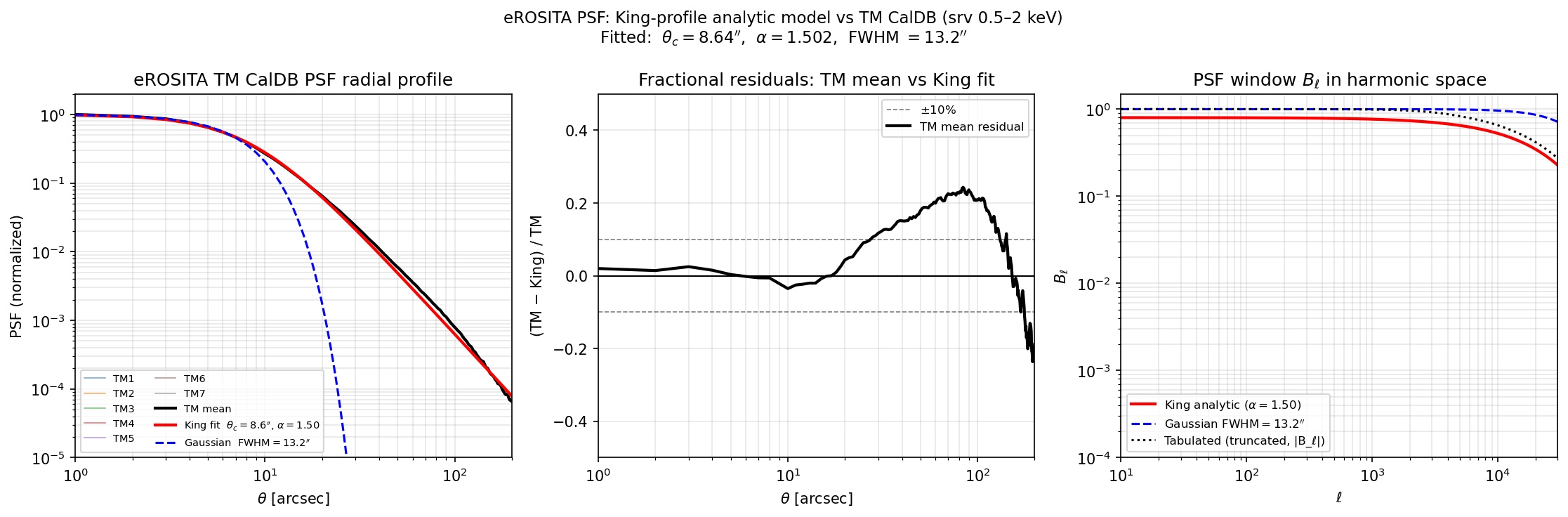
Figure PSF-1. Left: eROSITA TM1–TM7 radial PSF profiles (0.5–2 keV, CalDB srv-0500-2000) with King profile fit (\(\theta_c=8.64''\), \(\alpha=1.50\), red) and same-FWHM Gaussian (blue dashed). The King profile follows the power-law wings accurately while the Gaussian underestimates the PSF by orders of magnitude beyond \(\sim15''\). Centre: Fractional residuals (TM mean − King) / TM mean; within ±5% for \(\theta < 60''\), rising near the image boundary (240’’) where the tabulated CalDB data is truncated. Right: PSF window \(B_\ell\) in harmonic space. The Gaussian (blue) falls super-exponentially, suppressing all power above \(\ell\sim 200\); the King model (red) decays only as \(e^{-\ell\theta_c}\), preserving signal at high \(\ell\). The tabulated \(|B_\ell|\) (dotted) agrees with the analytic King at low \(\ell\); at high \(\ell\) the truncation causes numerical divergence that the analytic form avoids.

Validation figure generated by:

python -m hod_mod.scripts.galaxies.plot_erosita_psf
# Output: results/psf/erosita_psf_king_fit.png

Halo model cross-power spectra between galaxies and gas fields.

Provides HaloModelCrossSpectra which wraps a FullHaloModelPrediction instance and reuses its static cache (HMF, bias, DM profile FT, linear power spectrum) to compute:

• P_{g,y}(k) — galaxy × Compton-y (tSZ) cross-power, in (Mpc/h)².

• P_{m,y}(k) — matter × Compton-y cross-power (for lensing × tSZ), in (Mpc/h)².

• P_{g,X}(k) — galaxy × X-ray emissivity cross-power, in (Mpc/h)³ cm⁻⁶.

Projected observables:

• projected_gy() — Σ_y(r_p) [dimensionless Compton-y] via Abel projection.

• projected_gX() — w_{g,X}(r_p) via Abel projection.

• angular_cl_gy() — C_ℓ^{g,y} via Limber approximation.

• angular_cl_gX() — C_ℓ^{g,X} via Limber approximation.

References

Galaxy × tSZ formalism:

Pandey+2025, arXiv:2506.07432 — DES Year 3 shear × ACT DR6 tSZ Amodeo+2021, arXiv:2009.05557 — ACT × BOSS CMASS/LOWZ stacked tSZ

Galaxy × soft X-ray:

Comparat+2025, arXiv:2503.19796, A&A 697 A173

Pressure profile:

Arnaud+2010, arXiv:0910.1234 — A10 generalized NFW

Density profile:

Oppenheimer+2025, arXiv:2505.14782 — DPM

class hod_mod.observables.cross_spectra.HaloModelCrossSpectra(fhmp, pressure_profile: PressureProfileA10 | PressureProfileDPM | None = None, density_profile: GasDensityDPM | None = None, metallicity_profile=None, cooling_function=None, agn_model=None, ecf_gas_table=None, ecf_agn=None)

Bases: object

Halo model galaxy × gas cross-power spectra and projected observables.

Wraps a FullHaloModelPrediction and reuses its static cache (HMF, bias, DM profile FT, linear P(k)), adding gas-profile Fourier transforms for the y-field (tSZ) and X-ray emissivity field.

Parameters:

• fhmp (FullHaloModelPrediction) – Already-instantiated prediction object whose static cache is reused.

• pressure_profile (PressureProfileA10, optional) – Electron pressure profile for tSZ. If None, tSZ methods raise.

• density_profile (GasDensityDPM, optional) – Electron density profile for X-ray. If None, X-ray methods raise.

angular_cl_XX(ell_arr: ndarray, z_arr: ndarray, nz_X: ndarray, theta_cosmo: dict, psf_fwhm_arcsec: float | None = None, psf_king_theta_c_arcsec: float | None = None, psf_king_alpha: float = 1.5, return_components: bool = False, n_workers: int = 1, beta_gas: float | None = None, beta_pressure: float | None = None) → ndarray | dict

Angular auto-power spectrum C_ℓ^{X,X} of the total X-ray emission.

Includes the 1-halo and 2-halo gas–AGN cross-terms that vanish in angular_cl_gX() (which is exact and linear in X). See _pk_tables_XX() for the underlying P_{X,X}(k) decomposition.

\[C_\ell^{X,X} = \int_0^{\chi_{\max}} \frac{\mathrm{d}\chi}{\chi^2} W_X(\chi)^2\,P_{X,X}\!\left(k=\frac{\ell+\tfrac{1}{2}}{\chi}, z(\chi)\right)\]

Parameters:

• ell_arr ((Nell,) angular multipoles)

• z_arr ((Nz,) redshift array bracketing the X-ray source distribution)

• nz_X ((Nz,) X-ray window function (e.g. emissivity-weighted dV/dz,) – or a matched source dN/dz). Normalized internally like nz_g in angular_cl_gX(), but appears squared in the Limber integral since both legs of the correlation are the X-ray field.

• return_components (bool) – If True return {"total", "gas_gas", "cross", "agn_agn"}.

Returns:

cl_XX ((Nell,) or dict when return_components=True)

angular_cl_gX(ell_arr: ndarray, z_arr: ndarray, nz_g: ndarray, theta_cosmo: dict, hod_params: dict, psf_fwhm_arcsec: float | None = None, psf_king_theta_c_arcsec: float | None = None, psf_king_alpha: float = 1.5, return_components: bool = False, n_workers: int = 1, beta_gas: float | None = None, beta_pressure: float | None = None, agn_kwargs: dict | None = None, x_uk_override: list | ndarray | None = None) → ndarray | dict

Angular cross-power spectrum C_ℓ^{g,X} via the Limber approximation.

Identical structure to angular_cl_gy() but for the X-ray emissivity field (DPM Model). The returned spectrum has units of the emissivity power spectrum [(Mpc/h)³ cm⁻⁶] divided by χ² [(Mpc/h)²], giving [(Mpc/h) cm⁻⁶].

\[C_\ell^{g,X} = \int_0^{\chi_{\max}} \frac{\mathrm{d}\chi}{\chi^2} W_g(\chi)\,P_{g,X}\!\left(k=\frac{\ell+\tfrac{1}{2}}{\chi}, z(\chi)\right)\]

Parameters:

• ell_arr ((Nell,) angular multipoles)

• z_arr ((Nz,) redshift array bracketing the galaxy distribution)

• nz_g ((Nz,) dN/dz of the galaxy sample (normalized internally))

• theta_cosmo (cosmological parameters)

• hod_params (HOD parameters)

• psf_fwhm_arcsec (float | None) – eROSITA PSF FWHM [arcsec]. If given, multiply C_ℓ by the Gaussian PSF window B_ℓ = exp(−ℓ²σ²/2) (single-field convolution). Use 30.0 for the eROSITA soft X-ray PSF.

• psf_king_theta_c_arcsec (float | None) – King core radius [arcsec] for the analytic PSF window. If given, multiply C_ℓ by B_ℓ = exp(−ℓ θ_c) (α=3/2) or the general Bessel-K form. Fitted to eROSITA TM CalDB on-axis: 8.64”. Cannot be used together with psf_fwhm_arcsec.

• psf_king_alpha (float) – King slope for the analytic PSF window. Default 1.5.

• return_components (bool) – If True return a dict {"total", "gas", "agn"} instead of the total array.

• n_workers (int) – Number of threads for parallel evaluation of _pk_tables_gX at each redshift. -1 (default) uses os.cpu_count(). Set to 1 to disable parallelism. The z-points are independent, so thread-based parallelism is safe because JAX releases the GIL during computation.

Returns:

cl_gX ((Nell,) [(Mpc/h) cm⁻⁶] or dict when return_components=True)

angular_cl_gy(ell_arr: ndarray, z_arr: ndarray, nz_g: ndarray, theta_cosmo: dict, hod_params: dict, psf_fwhm_arcsec: float | None = None, psf_king_theta_c_arcsec: float | None = None, psf_king_alpha: float = 1.5) → ndarray

Angular cross-power spectrum C_ℓ^{g,y} via the Limber approximation.

Under Limber (Limber 1953; LoVerde & Afshordi 2008):

\[C_\ell^{g,y} = \int_0^{\chi_{\max}} \frac{\mathrm{d}\chi}{\chi^2} W_g(\chi)\,P_{g,y}\!\left(k=\frac{\ell+\tfrac{1}{2}}{\chi}, z(\chi)\right)\]

where \(W_g(\chi) = \mathrm{d}N_g/\mathrm{d}\chi\) (normalized). The y-field window is unity (already a LOS integral).

Parameters:

• ell_arr ((Nell,) angular multipoles)

• z_arr ((Nz,) redshift array for n(z) [must bracket the galaxy distribution])

• nz_g ((Nz,) dN/dz of the galaxy sample (will be normalized internally))

• theta_cosmo (cosmological parameters)

• hod_params (HOD parameters)

• psf_fwhm_arcsec (float | None) – If given, multiply C_ℓ by the Gaussian PSF window B_ℓ (single field).

• psf_king_theta_c_arcsec (float | None) – If given, multiply C_ℓ by the analytic King-profile PSF window B_ℓ = exp(−ℓ θ_c) for α=3/2, or the general Bessel-K form. Cannot be used together with psf_fwhm_arcsec.

• psf_king_alpha (float) – King slope for the analytic PSF window. Default 1.5.

Returns:

cl_gy ((Nell,) [(Mpc/h)²] (dimensionless after h-unit cancellation with χ²))

emissivity_xuk_bands_per_z(z_arr, theta_cosmo, hod_params, cooling_fns)

Multi-band version of emissivity_xuk_per_z() for the energy bands.

Computes the per-z, per-band raw emissivity FT X̃_b(k|M)/Λ_ref,b in one batched FT per z (GasDensityDPM.emissivity_full_uk_bands). Each band is divided by its OWN reference cooling Λ_ref,b = cooling_fns[b](1 keV, 0.3 Z⊙) so band b feeds angular_cl_gX(x_uk_override=...) exactly like the broad-band path (which divides by the broad-band Λ_ref).

Returns a list over z; each entry is a list over bands of (Nk, NM) arrays (so out[iz][b] is a valid x_uk_override for band b at z-index iz). self._dp/_pp/_mp must be set (the cooling tables are passed explicitly, not taken from self._cooling_fn).

emissivity_xuk_per_z(z_arr, theta_cosmo, hod_params)

Precompute the per-z raw emissivity FT X̃(k|M)/Λ_ref for the emulator.

Returns a list (one entry per z) of (Nk, NM) arrays — exactly what angular_cl_gX() consumes via x_uk_override. This isolates the expensive full-APEC FT (emissivity_full_uk, ~1.3 s/z) so a joint fit can cache it on a (p2, r_max) grid and skip it at evaluation time. The cached value is at this instance’s self._dp._ne_03; the caller scales by (n_e,0.3 / n_e,0.3_ref)² before passing it back.

Requires the full-APEC profiles (_dp/_pp/_mp/_cooling_fn).

projected_gX(rp_arr: ndarray, z: float, theta_cosmo: dict, hod_params: dict) → ndarray

Projected galaxy × X-ray emissivity w_{g,X}(r_p).

Same Abel projection as projected_gy() but for P_{g,X}(k). Units: (Mpc/h)³ cm⁻⁶ × (h/Mpc)² = (Mpc/h) cm⁻⁶. Multiply by the effective cooling function Λ_eff [erg cm³ s⁻¹] to compare to surface-brightness data.

Parameters:

• rp_arr ((NR,) [Mpc/h])

• z, theta_cosmo, hod_params (as for _pk_tables_gX)

Returns:

wgX ((NR,) [(Mpc/h) cm⁻⁶])

projected_gy(rp_arr: ndarray, z: float, theta_cosmo: dict, hod_params: dict) → ndarray

Projected galaxy × y signal Σ_y(r_p) [dimensionless Compton-y].

Computes the Abel projection of P_{g,y}(k):

\[\Sigma_y(r_p) = \frac{1}{2\pi^2} \int_0^\infty k\,P_{g,y}(k)\,J_0(k r_p)\,dk\]

Parameters:

• rp_arr ((NR,) projected separations [Mpc/h])

• z, theta_cosmo, hod_params (as for _pk_tables_gy)

Returns:

sigma_y ((NR,) [dimensionless])

hod_mod.observables.cross_spectra.psf_king_profile(theta_arcsec: ndarray, theta_c_arcsec: float = 8.64, alpha: float = 1.5) → ndarray

King-profile PSF in real (angular) space, normalized to 1 at θ=0.

PSF(θ) = (1 + (θ / θ_c)²)^{−α}

Parameters:

• theta_arcsec (angular separations [arcsec])

• theta_c_arcsec (King core radius [arcsec].) – Fitted to eROSITA TM CalDB (0.5–2 keV, on-axis): 8.64”.

• alpha (King slope (α > 1). Default 1.5 matches eROSITA TM fit.)

Returns:

PSF ((N,) array, in [0, 1])

hod_mod.observables.cross_spectra.psf_king_window_ell(ell_arr: ndarray, theta_c_arcsec: float = 8.64, alpha: float = 1.5) → ndarray

King-profile PSF window B_ℓ — analytic Hankel (Fourier-Bessel) transform.

Real-space PSF: PSF(θ) ∝ (1 + (θ/θ_c)²)^{−α}

Analytic Hankel transform (normalized to B_0 = 1):

\[B_\ell = \frac{2^{2-\alpha}}{\Gamma(\alpha-1)} (\ell\,\theta_c)^{\alpha-1}\,K_{\alpha-1}(\ell\,\theta_c)\]

where \(K_\nu\) is the modified Bessel function of the second kind.

Special case α = 3/2 → \(B_\ell = \exp(-\ell\,\theta_c)\), a pure exponential that is fully JAX-native.

Parameters:

• ell_arr ((Nell,) angular multipoles)

• theta_c_arcsec (King core radius [arcsec].) – Fitted to eROSITA TM CalDB (0.5–2 keV, on-axis): 8.64”. For a survey-averaged 30”-FWHM effective PSF use ~19.6”.

• alpha (King slope (α > 1). Default 1.5 matches eROSITA TM fit.)

Returns:

B_ell ((Nell,) dimensionless window function in [0, 1])

hod_mod.observables.cross_spectra.psf_window_ell(ell_arr: ndarray, fwhm_arcsec: float = 30.0) → ndarray

Gaussian PSF window function B_ℓ = exp(−ℓ² σ² / 2).

For a Gaussian PSF with FWHM = fwhm_arcsec arcseconds, the angular power spectrum of a PSF-convolved map is

\[C_\ell^{\rm obs} = C_\ell^{\rm true} \times B_\ell\]

where the galaxy field is not convolved (only the X-ray / y field). For the X-ray auto-power (if needed), multiply by B_ℓ².

Parameters:

• ell_arr ((Nell,) angular multipoles)

• fwhm_arcsec (PSF FWHM [arcsec], default 30 (eROSITA soft X-ray))

Returns:

B_ell ((Nell,) dimensionless window function in [0, 1])

—

X-ray AGN Model

(hod_mod.agn.xray)

XrayAGNModel models the mean soft X-ray (0.5–2 keV) AGN luminosity per dark-matter halo via an abundance-matching pipeline (Comparat et al. 2019, arXiv:1901.10866):

1. SHMR — maps \(M_h\) to \(\log_{10}M_*\) via smhm_girelli20() (Girelli et al. 2020). The double power-law relation is:

   \[\frac{M_*}{M_h}(z) = \frac{2A(z)}{(M_h/M_A)^{-\beta} + (M_h/M_A)^\gamma}\]

   with \(\log_{10}M_A = B + z\mu\), \(A(z) = C(1+z)^\nu\), \(\gamma(z) = D(1+z)^\eta\), \(\beta(z) = Fz + E\).

   The eight parameters (Girelli+2020 Table 3, best-fit without intrinsic scatter):

   Param	Default	Physical role	Evolution
   \(B\)	11.79	\(\log_{10}(M_A/M_\odot)\) at \(z=0\) — pivot halo mass where \(M_*/M_h\) peaks	\(\log_{10} M_A = B + z\mu\)
   \(\mu\)	0.20	Linear-\(z\) slope of pivot mass	—
   \(C\)	0.046	Peak \(M_*/M_h\) at \(z=0\) ≈ 4.6%	\(A(z) = C(1+z)^\nu\)
   \(\nu\)	−0.38	Redshift power-law of peak amplitude	—
   \(D\)	0.709	High-mass slope \(\gamma\) at \(z=0\)	\(\gamma(z) = D(1+z)^\eta\)
   \(\eta\)	−0.18	Redshift power-law of high-mass slope	—
   \(F\)	0.043	Linear-\(z\) coefficient of low-mass slope \(\beta\)	\(\beta(z) = Fz + E\)
   \(E\)	0.96	Low-mass slope at \(z=0\)	—

   A variant with 0.2 dex intrinsic scatter in \(M_*\) is available as hod_mod.connection.sham._GIRELLI20_SCATTER (Table 4 of Girelli+2020; pass B=11.83, mu=0.18, ... to smhm_girelli20()).

2. LX–M* polynomial — parametric fit to the hard-band (2–10 keV) XLF abundance-matching result:

   \[\log_{10} L_X^{\rm hard} = a + b\,(\log_{10}M_* - 10) + c\,(\log_{10}M_* - 10)^2\]

   Default: \(a=41.04,\ b=1.22,\ c=0\) (units: erg/s). Calibrated against the Hasinger+2005 LDDE soft XLF at \(z=0.1, 0.5, 1.0\) (joint 4-parameter fit; residuals \(<0.025\) dex at all three redshifts).

3. Band conversion — hard-to-soft (0.5–2 / 2–10 keV) flux ratio \(f_{h\to s}=0.35\) for a power-law SED with \(\Gamma=1.7\), \(N_H=10^{21}\,{\rm cm}^{-2}\) (Comparat+2019 §3.2 / Table 2).

4. Log-normal scatter — 0.8 dex scatter in \(\log_{10}L_X\) at fixed \(M_*\) boosts the ensemble mean by \(\exp(\sigma_{\rm dex}^2\,\ln^2 10\,/\,2)\).

5. Duty cycle \(f_{\rm DC}(z)\) — redshift-dependent active fraction, calibrated against the Hasinger+2005 LDDE evolution (\(p_1=3.97\)) and interpolated from six nodes:

   \(z\)	\(\log_{10} f_{\rm DC}\)
   0.00	−1.416
   0.25	−1.012
   0.75	−0.402
   1.75	−0.301
   3.50	−0.301
   10.1	−0.301

   The \(z\leq 0.75\) nodes follow a best-fit power-law \(10^{-1.416+4.171\log_{10}(1+z)}\); the higher-\(z\) nodes are capped at \(\log_{10}f_{\rm DC}=-0.301\) (\(f_{\rm DC}=0.50\)) because the unconstrained power-law extrapolation exceeds unity beyond \(z\approx 1.2\) (outside the Hasinger calibration range).

The combined mean luminosity per halo is:

\[\langle L_X^{\rm soft}(M_h, z)\rangle = f_{\rm DC}(z)\times 10^{\log_{10}L_X^{\rm hard}(M_*)}\times f_{h\to s} \times \exp\!\left(\frac{\sigma_{\rm dex}^2\,\ln^2 10}{2}\right)\]

Point-source profile: AGN are unresolved, so their real-space profile is a delta function and their Fourier transform is flat in \(k\):

\[\tilde{X}^{\rm AGN}(k|M) = \frac{\langle L_X^{\rm soft}(M,z)\rangle}{10^{43}}\]

This allows HaloModelCrossSpectra to include the AGN contribution alongside the thermal gas emission from GasDensityDPM.

Usage example:

import numpy as np
from hod_mod.agn.xray import XrayAGNModel

agn = XrayAGNModel()                            # Girelli+2020 SHMR, 0.8 dex scatter
m_halo = np.logspace(11, 15, 100)               # [Msun/h]
lx = agn.mean_agn_lx(m_halo, z=0.135)          # [erg/s]
log10_lx = agn.mean_agn_log10lx(m_halo, z=0.135)

# Pass to HaloModelCrossSpectra via the agn_model keyword:
from hod_mod.observables.cross_spectra import HaloModelCrossSpectra
from hod_mod.gas import GasDensityDPM

dp    = GasDensityDPM(model=2)
cross = HaloModelCrossSpectra(fhmp, density_profile=dp, agn_model=agn)
wgX   = cross.projected_gX(rp, z, theta_cosmo, hod_params)

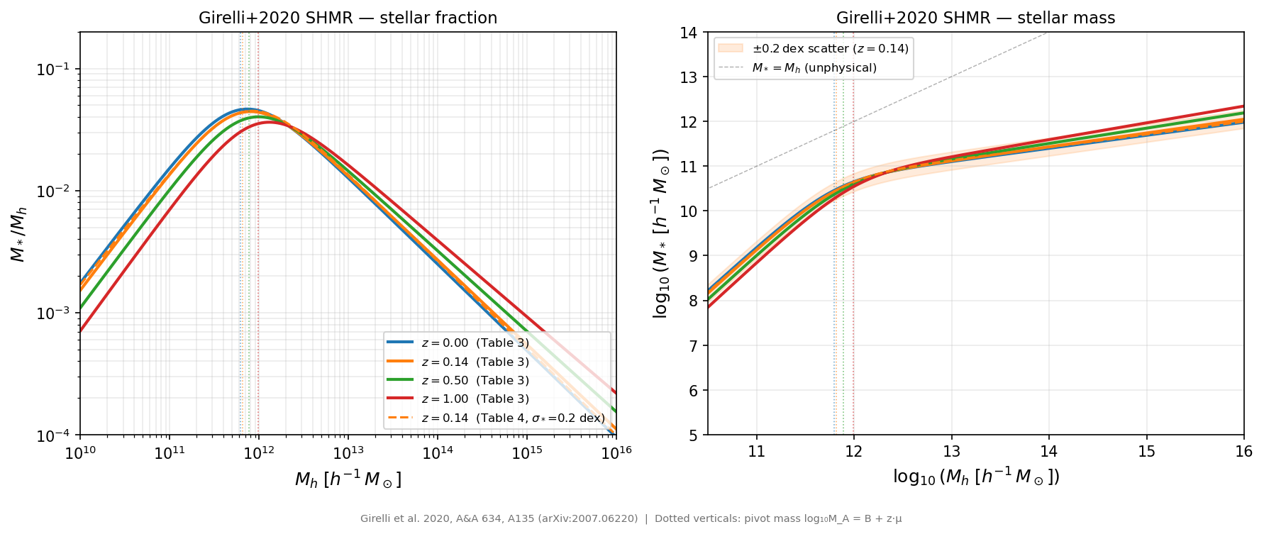
Figure AGN-1. Girelli+2020 SHMR: \(M_*/M_h\) ratio (left) and \(\log_{10}M_*\) (right) vs \(\log_{10}M_h\) at \(z=0, 0.14, 0.5, 1.0\). Dashed line shows the scatter-fit variant (Table 4). Shaded band: ±0.2 dex intrinsic scatter at \(z=0.14\). Dotted verticals: pivot halo mass \(M_A(z)\).

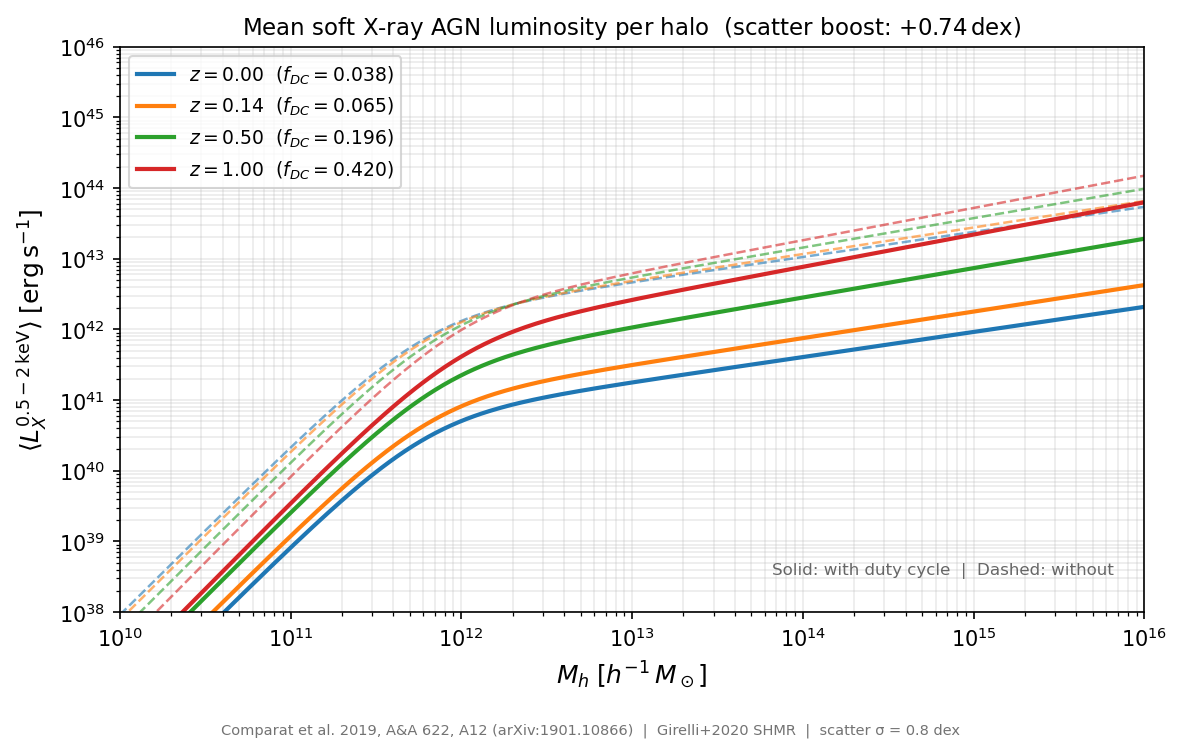
Figure AGN-2. Mean soft X-ray AGN luminosity \(\langle L_X^{0.5-2\,{\rm keV}}\rangle\) vs \(\log_{10}M_h\) at four redshifts. Solid curves include the duty cycle \(f_{\rm DC}(z)\); dashed curves show the pre-duty-cycle luminosity, illustrating the redshift-dependent suppression and the +0.74 dex scatter boost.

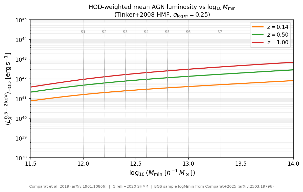
Figure AGN-3. HOD-weighted mean AGN luminosity \(\langle L_X\rangle_{\rm HOD}\) vs HOD threshold \(\log_{10}M_{\min}\) at \(z=0.14, 0.5, 1.0\) (Tinker+2008 HMF, \(\sigma_{\log m}=0.25\)). Dotted verticals label the seven BGS stellar-mass samples (S1–S7) of Comparat+2025.

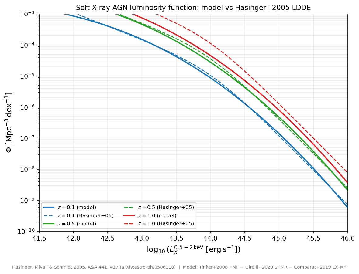
Figure AGN-4. Predicted soft X-ray (0.5–2 keV) AGN luminosity function (solid) vs the Hasinger+2005 LDDE reference (dashed, arXiv:astro-ph/0506118) at \(z=0.1, 0.5, 1.0\). Predicted curves integrate the Tinker+2008 HMF with the Girelli+2020 SHMR, LX–M* relation, 0.8 dex log-normal scatter, and the calibrated redshift-dependent duty cycle. Both parameters and duty cycle were jointly fitted to match this reference; residuals are \(<0.025\) dex at all three redshifts.

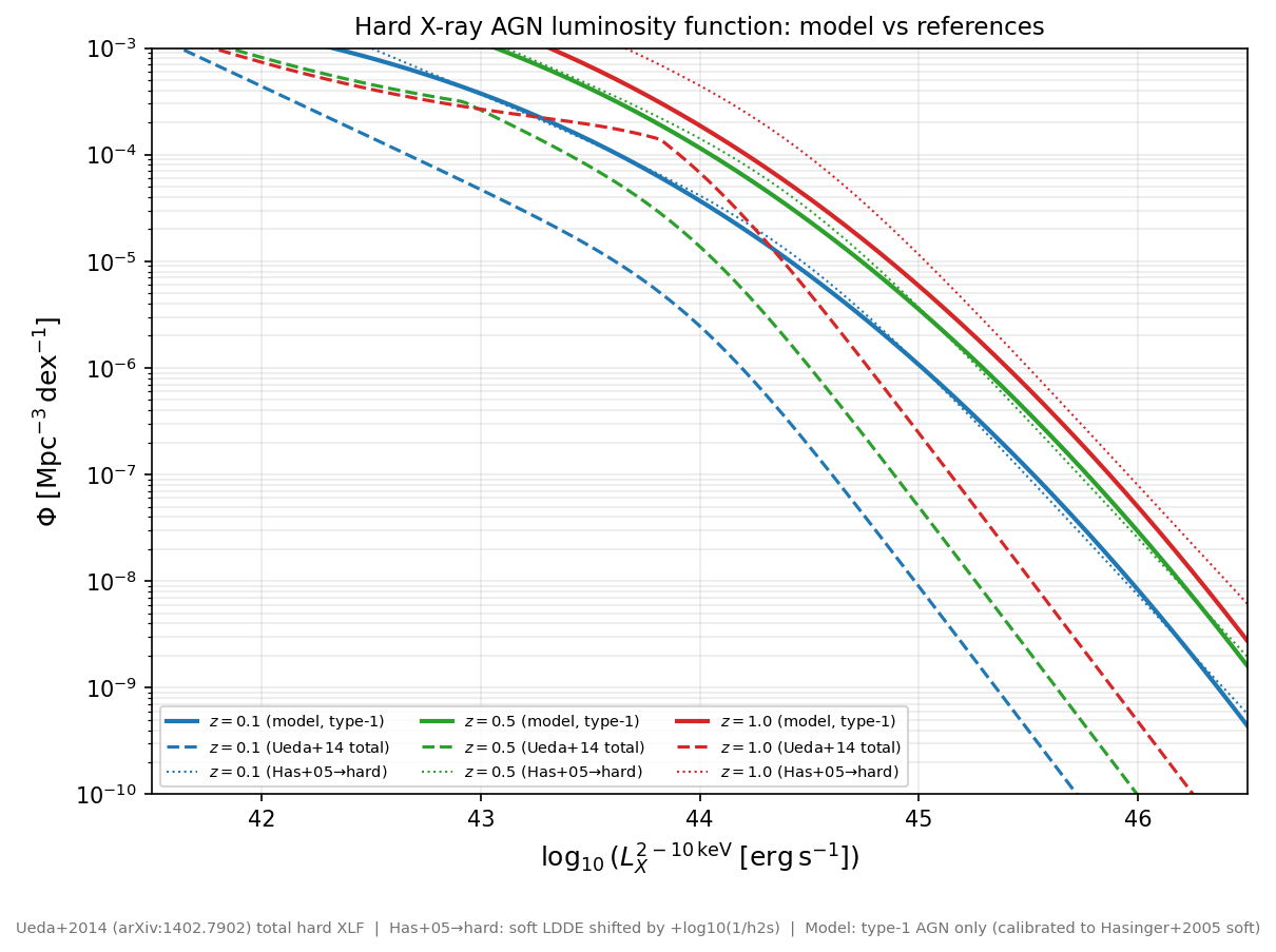
Figure AGN-5. Predicted hard X-ray (2–10 keV) AGN luminosity function (solid, type-1 AGN only) at \(z=0.1, 0.5, 1.0\), with two references: Ueda+2014 LDDE (dashed, arXiv:1402.1836) — total hard XLF including obscured (type 2) and Compton-thick AGN; Hasinger+2005 → hard (dotted) — the soft LDDE shifted to the hard band via \(\log_{10}L_{\rm hard}=\log_{10}L_{\rm soft}-\log_{10}f_{h\to s}\), representing type-1-only AGN. The model lies between the two references: calibrated to the soft (type-1) XLF, it reproduces the type-1-only hard XLF and sits \(\sim 3\)–\(5\times\) below Ueda+2014 at \(L<10^{44}\) — consistent with the observed \(\sim 70\%\) obscured fraction at these luminosities.

References: Comparat et al. 2019 (arXiv:1901.10866); Girelli et al. 2020 (arXiv:2007.06220); Hasinger, Miyaji & Schmidt 2005 (arXiv:astro-ph/0506118) — soft XLF LDDE reference; Ueda et al. 2014 (arXiv:1402.1836) — total hard XLF LDDE reference.

X-ray AGN model following Comparat+2019 abundance matching, implemented in JAX.

Provides XrayAGNModel which maps dark-matter halo mass to a mean soft X-ray (0.5–2 keV) AGN luminosity via:

1. SHMR — any callable M_halo → log10(M_*) (e.g. smhm_girelli20())

2. LX–M_* relation — parametric fit to the Comparat+2019 abundance-matching result (HAM of the hard-band XLF with the SHMR): log10(L_X^{2-10 keV}) = a + b × (log10 M_* − 10) + c × (log10 M_* − 10)²

3. Band conversion — hard-to-soft (0.5–2 / 2–10 keV) flux ratio from Comparat+2019 Table 2

4. Log-normal scatter — 0.8 dex in LX at fixed M_* → boost factor on mean ⟨L_X⟩

5. Duty cycle — f_DC(z) from Comparat+2019 Table 1 interpolation

The class provides:

• mean_agn_lx() — mean soft-band L_X(M_halo, z) including duty cycle

• agn_emissivity_uk() — Fourier transform of the AGN contribution to the X-ray surface brightness (point-source, flat in k-space)

Both methods are fully differentiable with JAX.

References

Comparat et al. 2019, A&A 622, A12 (arXiv:1901.10866)

class hod_mod.agn.xray.XrayAGNModel(shmr_func=None, scatter_lx: float = 0.8, f_sat_agn: float = 0.1, lx_a: float = 41.04, lx_b: float = 1.22, lx_c: float = 0.0, hard_to_soft: float = 0.35)

Bases: object

X-ray AGN model following Comparat+2019 abundance matching.

Connects dark-matter halo mass to mean soft X-ray AGN luminosity via stellar-to-halo mass relation (SHMR) + LX–M* HAM relation with log-normal scatter and a redshift-dependent duty cycle.

The model is fully JAX-differentiable: all array computations use jnp.

Parameters:

• shmr_func (callable(log10m_halo, z, **shmr_params) → log10(M_ [M_sun])*) – SHMR function. Should accept JAX arrays and return a JAX array. The default is smhm_girelli20().

• scatter_lx (float) – Log-normal scatter in log10 L_X at fixed log10 M_* [dex]. Default 0.8.

• f_sat_agn (float) – Fraction of AGN that are satellites (default 0.1).

• lx_a, lx_b, lx_c (float) – Coefficients of the LX–M_* polynomial (see _lx_hard_mean()).

Notes

The mean luminosity per halo already includes the scatter boost: ⟨L_X^{soft}⟩ = f_DC(z) × 10^{log10_L_hard} × hard_to_soft × exp(σ² / 2)

The AGN contribution to P_{g,X}(k) is a point-source (delta function in real space), so X̃^{AGN}(k|M) is flat in k at the value ⟨L_X^{soft}⟩.

agn_emissivity_uk(k_arr: Array, m_halo_arr: Array, z: float, theta_cosmo: dict, shmr_params: dict | None = None) → Array

Fourier transform of the AGN X-ray emissivity contribution.

AGN are point sources, so their 3D profile is a delta function. The Fourier transform is flat in k:

\[\tilde{X}^{\rm AGN}(k|M) = \frac{\langle L_X^{\rm AGN}(M) \rangle} {4\pi D_L^2(z)} \times (1+z)^2 \times f_{\rm surf}\]

The array is normalized by 1e43 to keep float32-safe magnitudes. _pk_tables_gX() applies 1e43 / (Lambda_eff × (cm_per_Mpc_h)³) to convert P_gX_agn into (Mpc/h)³ cm⁻⁶, matching the gas emissivity units.

Parameters:

• k_arr ((Nk,) [h/Mpc] — wavenumber array (output shape driver))

• m_halo_arr ((NM,) [Msun/h])

• z (redshift)

• theta_cosmo (dict with ‘h’, ‘Omega_m’)

• shmr_params (dict, optional)

Returns:

uk_agn ((Nk, NM) [L_X / 1e43, dimensionless] — flat in k (point-source AGN))

mean_agn_log10lx(m_halo_arr, z: float, shmr_params: dict | None = None) → ndarray

log10 of the mean soft X-ray AGN luminosity per halo [erg/s].

Stays in log-space to avoid float32 overflow (L_X ~ 10^{42-44} erg/s exceeds the float32 maximum of ~3.4×10^{38}).

Returns:

log10_lx_soft ((NM,) float64 ndarray)

mean_agn_lx(m_halo_arr: Array, z: float, shmr_params: dict | None = None) → ndarray

Mean soft X-ray AGN luminosity ⟨L_X^{0.5-2 keV}⟩ per halo [erg/s].

Includes duty cycle and scatter boost but not the point-to-point scatter (which only affects the variance, not the mean in the halo model).

Parameters:

• m_halo_arr ((NM,) [Msun/h] — halo mass)

• z (redshift)

• shmr_params (dict, optional — extra kwargs forwarded to the SHMR function)

Returns:

lx_soft ((NM,) float64 ndarray [erg/s])

HAM AGN Model

(hod_mod.agn.ham)

HamAGNModel implements the Comparat et al. 2019 abundance-matching (HAM) AGN model. Unlike XrayAGNModel, which uses a parametric \(L_X\)–\(M_*\) relation, this model matches the cumulative galaxy number density to the hard X-ray luminosity function directly, so the hard XLF is reproduced by construction. The soft XLF is then predicted via the obscuration model and K-corrections.

Pipeline

1. SHMR — Zu & Mandelbaum (2015) Eq. 19 maps each halo mass \(M_h \to M_*\) (bisection inversion, 60 iterations).

2. HAM — Cumulative densities are matched:

   \[f_{\rm DC}(z)\,n_{\rm gal}(>M_*) = n_{\rm AGN}(>L_X^{\rm hard})\]

   using either the Aird et al. 2015 LADE or the Ueda et al. 2014 LDDE hard XLF. A 2D lookup table \((z, \log M_h) \to \log L_X^{\rm hard}\) is precomputed at instantiation (~12 s).

3. Obscuration model — Comparat+2019 eqs. 4–11 assign type-1, type-2, and Compton-thick fractions as a function of \(L_X^{\rm hard}\) and \(z\).

4. K-correction — The tabulated \(f_{\rm obs}(z, \log N_H)\) converts rest-frame 2–10 keV to observed 0.5–2 keV luminosity. The table is bundled in the package at hod_mod/data/agn/ and loaded automatically (no environment variables required).

K-correction table

The table encodes

\[f_{\rm obs}(z,\log N_H) = \frac{L_X^{0.5\text{–}2\,\mathrm{keV},\,\mathrm{obs}}} {L_X^{2\text{–}10\,\mathrm{keV},\,\mathrm{RF,\,intrinsic}}}\]

computed with XSPEC using the spectral model TBabs(plcabs + zgauss + constant×powerlaw + pexrav×constant) with photon index \(\Gamma = 1.9\), scattered fraction \(f_{\rm scat} = 0.02\), and Galactic column \(N_H^{\rm gal} = 3\times10^{20}\ \mathrm{cm}^{-2}\) (solar abundances; Wilms, Allen & McCray 2000). The model includes photoelectric absorption (TBabs), Compton-thick transmission (plcabs), an iron-K emission line (zgauss), reflection (pexrav), and a scattered power-law component. The grid covers 13 redshifts (\(z = 0\text{–}6\), step 0.5) and 13 column densities (\(\log N_H = 20\text{–}26\), step 0.5). Key normalisation values: \(f_{\rm obs}(z=0, \log N_H=20) = 0.607\) (unobscured; includes Galactic absorption and reflection) and \(f_{\rm obs}(z=0, \log N_H\geq24) = 0.0133\) (Compton-thick floor; scattered component only).

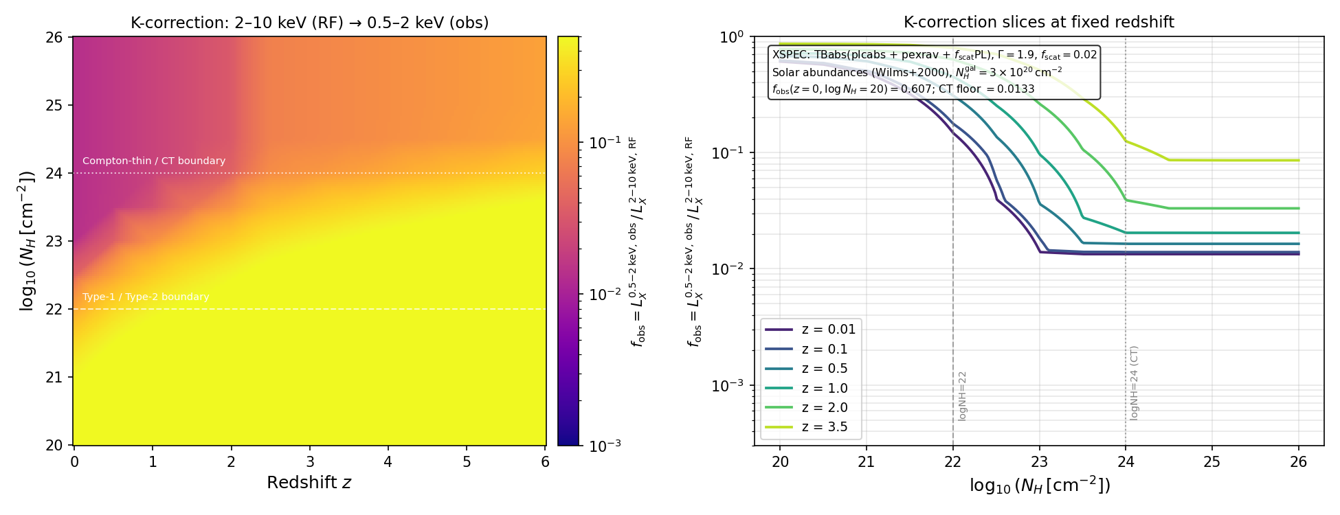
Figure HAM-0. X-ray K-correction grid computed with XSPEC. Left: \(f_{\rm obs}\) in the \((z, \log N_H)\) plane (logarithmic colour scale). The dashed line marks the type-1/type-2 boundary at \(\log N_H = 22\); the dotted line marks the Compton-thin/Compton-thick boundary at \(\log N_H = 24\). Right: Slices at fixed redshift. The plateau above \(\log N_H = 24\) at \(f_{\rm obs} \approx 0.0133\) is the scattered-light component that passes through the absorbing column.

HAM mapping and XLF reproduction

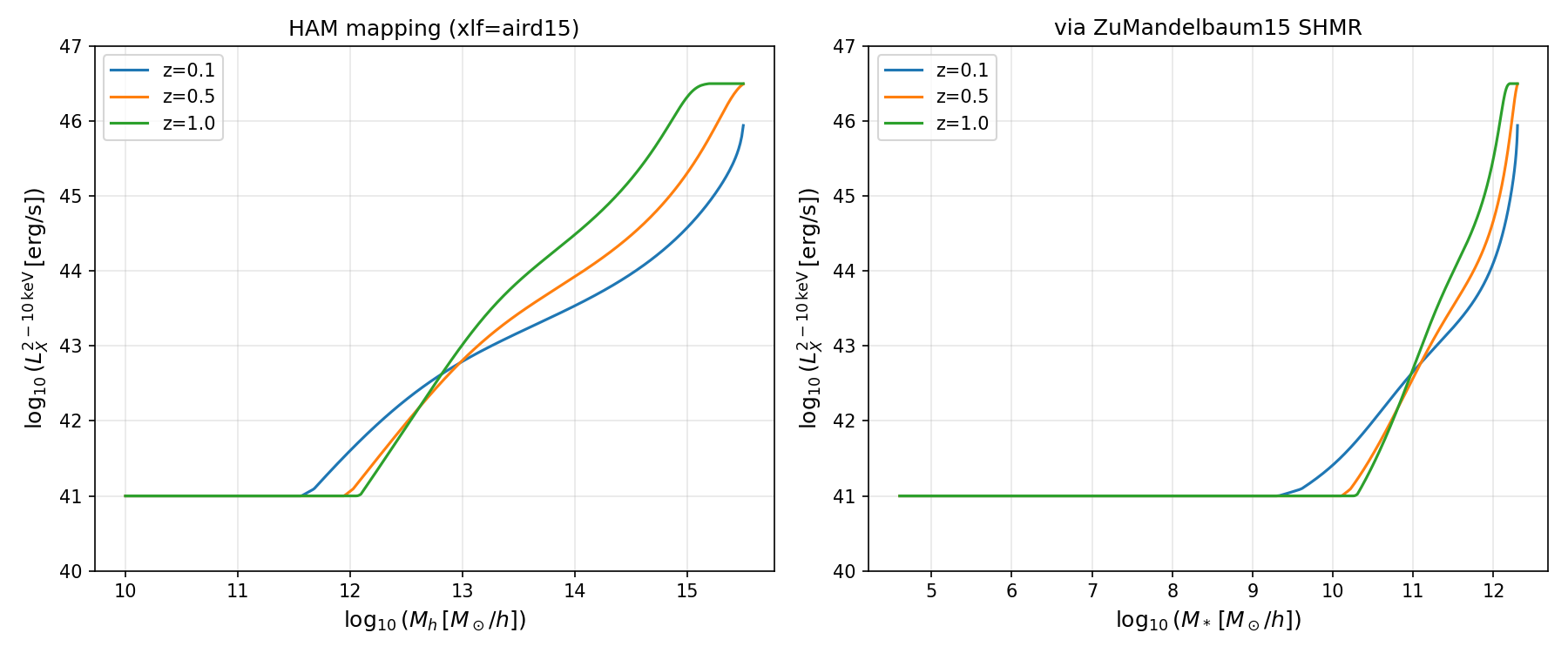
Figure HAM-1. HAM luminosity mapping. Left: \(\log L_X^{\rm hard}\) vs. halo mass at \(z = 0.1, 0.5, 1.0\). Halos below \(\log M_h \approx 12\) are assigned the grid lower boundary (\(10^{41}\) erg/s); at those masses the galaxy occupation is negligible so the value does not affect cross-correlation predictions. Right: Same mapped through the Zu & Mandelbaum (2015) SHMR to stellar mass.

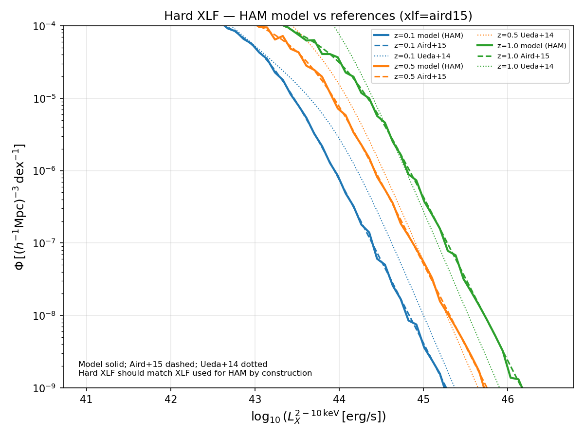
Figure HAM-2. Hard (2–10 keV) XLF check. Solid lines show the HAM-predicted XLF (recovered by binning the HAM table against the halo mass function); dashed lines show the input Aird+2015 LADE; dotted lines show Ueda+2014 LDDE. The model reproduces the input XLF by construction over the range \(10^{43}\) – \(10^{45.5}\) erg/s.

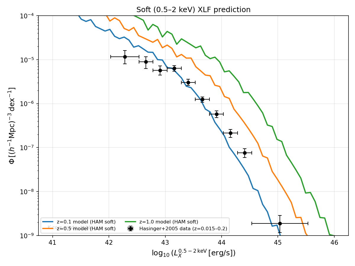
Figure HAM-3. Predicted soft (0.5–2 keV) XLF (solid) compared with Hasinger, Miyaji & Schmidt (2005) LDDE (dashed) at \(z = 0.1, 0.5, 1.0\). The model lies ~0.5–1 dex below Hasinger at the bright end because obscured sources are redistributed to fainter apparent soft luminosities.

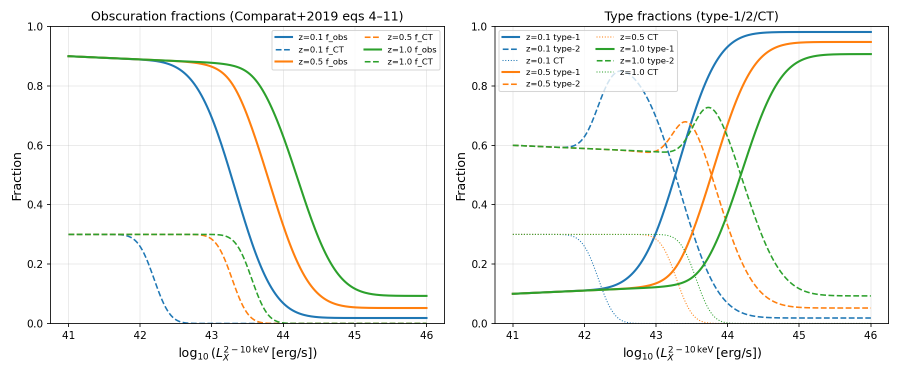
Figure HAM-4. Obscuration fractions (Comparat+2019 eqs. 4–11). Left: Total obscured (\(\log N_H > 22\)) and Compton-thick fractions as a function of \(L_X^{\rm hard}\). Right: Type-1, type-2, and CT fractions.

AGN model validation

The following figures compare model predictions against literature data for three complementary AGN statistics. All predictions are derived analytically from the HAM table: the Tinker+2008 HMF is weighted by the HAM \(L_X(M_h, z)\) mapping and the Zu & Mandelbaum (2015) SHMR, convolved with a 0.8 dex log-normal scatter in \(L_X\) at fixed \(M_h\). Only halos with a genuine HAM assignment (\(\log L_X > 41.05\)) are included; lower-mass halos are clamped to the XLF floor and excluded.

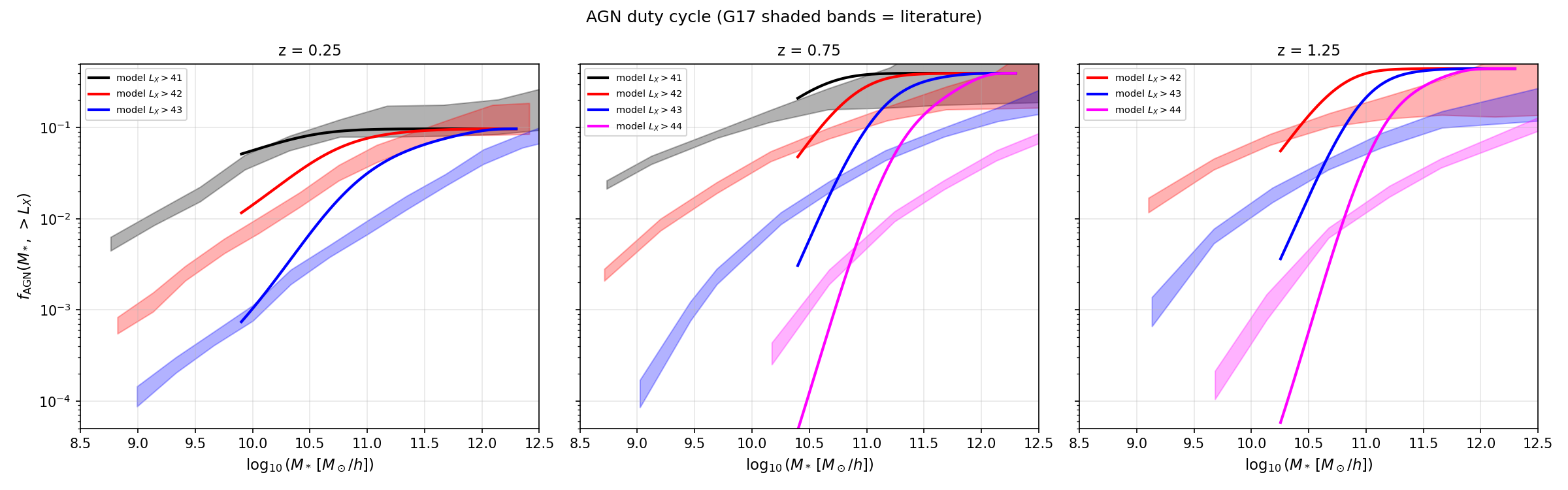
Figure HAM-5. AGN duty cycle \(f_{\rm AGN}(M_*, > L_X)\) at \(z = 0.25, 0.75, 1.25\) for hard-band luminosity thresholds \(\log L_X > 41, 42, 43\) (and 44 at \(z \geq 0.75\)). Shaded bands show Georgakakis et al. (2017, G17) observational constraints; stellar masses are shifted by \(\Delta\log M_* = \log_{10}(0.6777^2)\) to convert from the \(h = 0.6777\) convention used by G17.

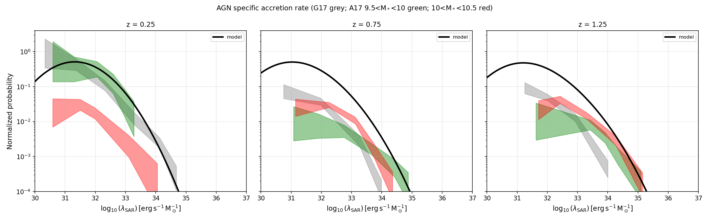
Figure HAM-6. Specific black-hole accretion rate (LSAR) distribution \(p(\log\lambda_{\rm SAR})\) at \(z = 0.25, 0.75, 1.25\). The model curve (black) is a Gaussian-kernel-smoothed sum over the HMF, with \(\lambda_{\rm SAR} = L_X^{\rm hard}/M_*\) (erg s⁻¹ M_⊙⁻¹). Grey shading: Georgakakis et al. (2017) constraints for all stellar masses. Green and red shading: Aird et al. (2018, A18) mass bins \(9.5 < \log M_* < 10\) and \(10 < \log M_* < 10.5\), respectively.

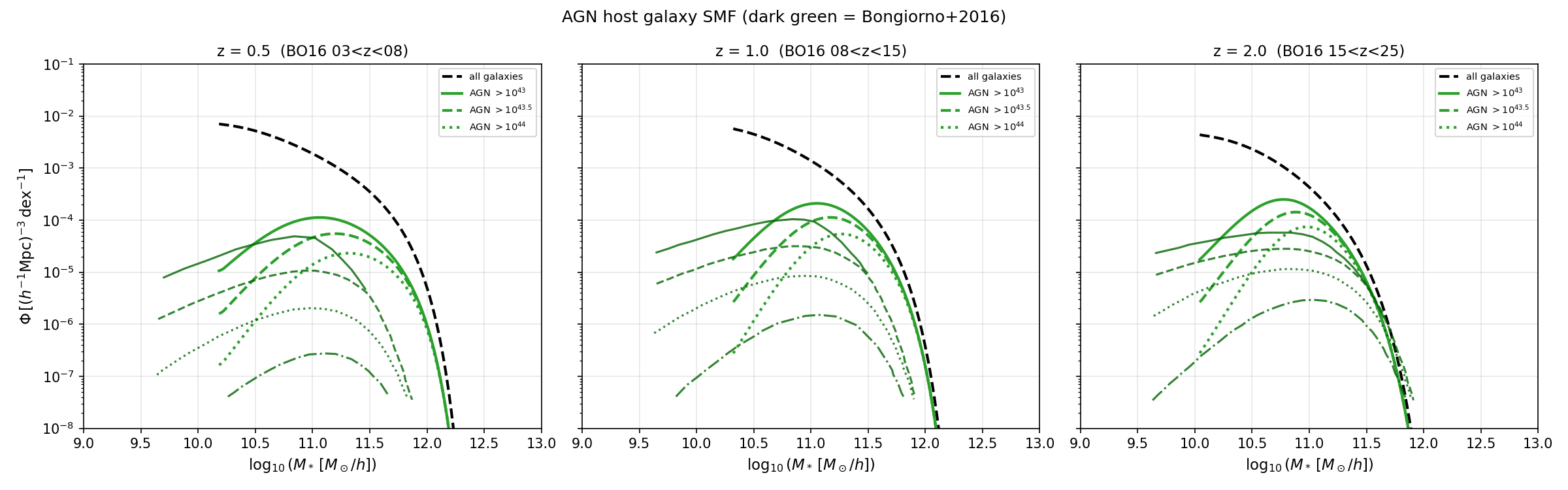
Figure HAM-7. AGN host galaxy stellar mass function \(\Phi(M_*)\) at \(z \approx 0.5, 1.0, 2.0\) for three hard-band luminosity thresholds (\(\log L_X > 43, 43.5, 44\)). Dashed black: total galaxy SMF from the Zu & Mandelbaum (2015) SHMR Jacobian. Dark-green curves: Bongiorno et al. (2016, BO16) AGN host galaxy SMF from COSMOS.

Validation references: Georgakakis et al. 2017, MNRAS 471, 1976 — AGN duty cycle and LSAR; Aird et al. 2018, MNRAS 474, 1225 — specific accretion rate distributions; Bongiorno et al. 2016, A&A 586, A78 — AGN host galaxy SMF.

Usage

from hod_mod.agn.ham import HamAGNModel
import numpy as np

# Instantiate — K-correction table loaded from package data automatically
agn = HamAGNModel(xlf="aird15")          # or xlf="ueda14"

m_halo = np.array([1e12, 1e13, 1e14])    # M_sun/h
lx_soft = agn.mean_agn_lx(m_halo, z=0.5)        # erg/s, 0.5-2 keV
log10lx = agn.mean_agn_log10lx(m_halo, z=0.5)

# Pass to HaloModelCrossSpectra
from hod_mod.observables.cross_spectra import HaloModelCrossSpectra
cross = HaloModelCrossSpectra(fhmp, density_profile=dp, agn_model=agn)

References: Comparat et al. 2019 (arXiv:1901.10866); Aird et al. 2015 (arXiv:1503.01120) — LADE hard XLF; Ueda et al. 2014 (arXiv:1402.1836) — LDDE hard XLF; Zu & Mandelbaum 2015 (arXiv:1505.02781) — iHOD SHMR; Hasinger, Miyaji & Schmidt 2005 (arXiv:astro-ph/0506118) — soft XLF LDDE reference; Wilms, Allen & McCray 2000, ApJ 542, 914 — X-ray absorption cross-sections.

HAM-based X-ray AGN model following Comparat+2019.

Implements HamAGNModel which abundance-matches galaxy stellar masses (from the Zu & Mandelbaum 2015 SHMR + halo mass function) to hard X-ray luminosities drawn from the Aird+2015 LADE or Ueda+2014 LDDE XLF.

Pipeline

1. SHMR — Zu & Mandelbaum (2015) Eq. 19 maps M_halo → M_* for centrals.

2. HAM — Cumulative n_gal(>M_*) × f_DC = n_AGN(>L_X) is matched to the Aird+2015 or Ueda+2014 XLF to assign L_X^{hard} to each halo. Precomputed at init time over a 2D grid (z, log10 M_halo).

3. Obscuration model — Comparat+2019 eqs 4–11 assign type fractions (Compton-thick, type-2, type-1) as a function of L_X^{hard} and z.

4. K-correction — Tabulated fraction_observed(z, logNH) from v3_fraction_observed_A15_RF_hard_Obs_soft_fscat_002.txt converts the hard-band luminosity to an effective soft-band (0.5–2 keV) signal. Falls back to simplified f_unobs × h2s when the table is unavailable.

The hard XLF is reproduced by construction; the soft XLF is predicted.

The class exposes the same interface as XrayAGNModel so it plugs into HaloModelCrossSpectra without modification.

References

Comparat et al. 2019, A&A 622, A12 (arXiv:1901.10866) Aird et al. 2015, ApJ 815, 66 (arXiv:1503.01120) — LADE hard XLF Ueda et al. 2014, ApJ 786, 104 (arXiv:1402.7902) — LDDE total hard XLF Zu & Mandelbaum 2015, MNRAS 454, 1161 (arXiv:1505.02781) — iHOD SHMR

class hod_mod.agn.ham.HamAGNModel(pk_lin=None, theta_cosmo: dict | None = None, zu15_shmr_params: dict | None = None, scatter_lx: float = 0.8, f_sat_agn: float = 0.1, duty_cycle: float | None = None, xlf: str = 'aird15', kcorr_path: str | None = None, hmf=None)

Bases: object

Comparat+2019 HAM AGN model.

Abundance-matches galaxy stellar masses (from the Zu & Mandelbaum 2015 SHMR) to hard X-ray luminosities from the Aird+2015 or Ueda+2014 XLF. The hard XLF is reproduced by construction; the soft XLF follows from the obscuration model and K-corrections.

Parameters:

• pk_lin (LinearPowerSpectrum, optional) – Linear power spectrum instance. Used to build the HMF for the HAM precomputation. If None, a default Planck-2018 instance is created.

• theta_cosmo (dict, optional) – Cosmology dictionary (same format as LinearPowerSpectrum.default_cosmology()). Default: Planck 2018.

• zu15_shmr_params (dict, optional) – Kwargs for _mstar_from_mh_zu15(). Default: Zu & Mandelbaum (2015) Table 2 best-fit values for the SDSS volume-limited sample.

• scatter_lx (float) – Log-normal scatter in log10(L_X) at fixed M_halo [dex]. Default 0.8.

• f_sat_agn (float) – Fraction of satellite galaxies hosting AGN. Default 0.10.

• duty_cycle (float or None) – Fixed duty cycle f_DC. If None (default), f_DC(z) is interpolated from the Comparat+2019 table.

• xlf ({‘aird15’, ‘ueda14’}) – Hard XLF reference. 'aird15' (default): Aird+2015 LADE (Comparat+2019 parametric form). 'ueda14': Ueda+2014 LDDE.

• kcorr_path (str or None) – Path to the K-correction table v3_fraction_observed_A15_RF_hard_Obs_soft_fscat_002.txt. Resolution order:

  1. kcorr_path argument

  2. $GIT_STMOD_DATA/data/models/model_AGN/xray_k_correction/v3_fraction_observed_A15_RF_hard_Obs_soft_fscat_002.txt

  3. Simplified fallback: k_eff = f_unobs × h2s (with a warning).

agn_emissivity_uk(k_arr, m_halo_arr, z: float, theta_cosmo: dict, shmr_params: dict | None = None, *, scatter_lx: float | None = None, log10_A_kcorr: float = 0.0, log10_A_dc: float = 0.0) → ndarray

Fourier transform of the AGN X-ray emissivity (point-source, flat in k).

Same interface and units as agn_emissivity_uk().

Returns:

uk_agn ((Nk, NM) float64 ndarray [L_X / 1e43, dimensionless])

ham_log10lx_hard(log10_mh: ndarray, z: float) → ndarray

Raw HAM hard-band luminosity at given halo masses.

No scatter, no obscuration, no duty-cycle correction.

Parameters:

• log10_mh (log10(M_h / [M_sun/h]) array)

• z (redshift)

Returns:

log10_lx_hard (log10(L_X^{2-10 keV} / erg/s))

mean_agn_log10lx(m_halo_arr, z: float, shmr_params: dict | None = None, *, scatter_lx: float | None = None, log10_A_kcorr: float = 0.0, log10_A_dc: float = 0.0) → ndarray

log10 of the mean soft X-ray AGN luminosity per halo [erg/s].

Includes: HAM hard luminosity + scatter boost + K-correction (obscuration-weighted) + duty cycle.

Parameters:

• m_halo_arr ((NM,) array [M_sun/h])

• z (redshift)

• shmr_params (ignored (retained for interface compatibility))

• scatter_lx (optional override of the constructor’s scatter_lx) – (dex), used to recompute the scatter boost on the fly. Cheap: unlike duty_cycle, scatter never feeds into the precomputed HAM table, so this does not retrigger the ~12s precompute.

• log10_A_kcorr (log10 multiplicative rescaling of the effective) – K-correction k_eff, clamped so the result never exceeds 1 (k_eff is a flux fraction). Default 0.0 = no change.

• log10_A_dc (log10 multiplicative rescaling of the duty cycle used) – in this population-averaging step ONLY, clamped at 1. This deliberately does not alter the duty cycle baked into the abundance-matching table (ham_log10lx_hard / HAM precompute) — re-deriving that self-consistently would require rebuilding the table per trial value. Default 0.0 = no change. See _precompute_ham() for the two distinct roles duty cycle plays in this model.

Returns:

log10_lx_soft ((NM,) float64 ndarray [erg/s])

mean_agn_lx(m_halo_arr, z: float, shmr_params: dict | None = None, *, scatter_lx: float | None = None, log10_A_kcorr: float = 0.0, log10_A_dc: float = 0.0) → ndarray

Mean soft X-ray AGN luminosity per halo [erg/s].

hod_mod.agn.ham.kcorr_at(kcorr_interp, kcorr_mode: str, z: float, lognh: float) → float

K-correction fraction at (z, logNH). Returns h2s if table unavailable.

hod_mod.agn.ham.mean_k_eff(kcorr_interp, kcorr_mode: str, log10_lx_hard: ndarray, z: float) → ndarray

Effective soft K-correction averaged over the N_H type distribution.

hod_mod.agn.ham.obscured_fraction(log10_lx: Array, z: float) → Array

Total obscured fraction logNH > 22 (type-2 + CT) — Comparat+2019 eq. 11.

Returns values in [0, 1]. All operations use jnp (JIT-compatible).

hod_mod.agn.ham.setup_kcorrection(kcorr_path: str | None = None)

Resolve the K-correction table and build the interpolator.

Resolution order: kcorr_path argument → package data/agn/ → $GIT_STMOD_DATA → simplified fallback.

Returns:

(interp, mode) ((LinearNDInterpolator or None, {‘table’, ‘simplified’})) – interp maps (z, logNH) → fraction_observed; mode is 'table' when the table loaded successfully, else 'simplified'.

—

HOD AGN Model

(hod_mod.agn.hod)

HODAgnModel is a third AGN model that places AGN with an explicit halo occupation distribution (a constant-duty-cycle More+2015 form, MoreConstFincHODModel), maps host halo masses to stellar masses with the Zu & Mandelbaum 2015 SHMR, and assigns \(L_X\) by a flux/optically-selected abundance match against the Aird+2015 XLF. Unlike XrayAGNModel and HamAGNModel, it exposes its own AGN occupation nc_ns_agn which drives an occupation-weighted X-ray auto/cross power spectrum (Lau et al. 2024, arXiv:2410.22397, App. A). See Zu & Mandelbaum 2015 iHOD Model — SDSS, X-ray & BGS (HOD AGN model rubric) for the full description and the LS10-BGS S1…S7 sample configuration.

HOD-based X-ray AGN model with modified abundance matching.

This is a third AGN X-ray model, conceptually distinct from HamAGNModel (which abundance-matches halo mass directly to L_X) and XrayAGNModel (a parametric L_X(M_*)). Here AGN are placed by an explicit halo occupation distribution and their luminosities are assigned by abundance matching against a flux/optically-selected X-ray luminosity function.

Pipeline

1. AGN HOD — a simple 5-parameter More+2015 occupation with a constant duty cycle f_inc (mass-independent), see MoreConstFincHODModel. This populates halos with central and satellite AGN.

2. Stellar masses — the Zu & Mandelbaum (2015) SHMR turns the AGN-host halo masses into a stellar-mass distribution (centrals and satellites).

3. Modified abundance matching at the sample mean redshift z_mean:

   • Build the luminosity distribution from the XLF (Aird+2015 by default) down to log10lx_min (1e39 erg/s).

   • Convert hard-band L_X to observed soft (0.5–2 keV) luminosity via the obscuration-weighted K-correction, then to observed flux FX with the luminosity distance.

   • Predict the r-band magnitude r_mag = a + b*log10(FX) (default a, b = -7, -2) and keep 16 ≤ r_mag ≤ 19.5.

   • Rank-order match the selected L_X distribution onto the (f_inc-suppressed) AGN-host stellar-mass distribution. Because f_inc is applied to the host population, the matched abundances agree mechanically — no rescaling of flux or luminosity is applied.

   The matching is performed deterministically on cumulative number densities (the noise-free limit of drawing a finite Monte-Carlo array; the sample volume cancels and only enters the absolute-count diagnostics).

4. Outputs — independent AGN occupations N_cen(AGN), N_sat(AGN), a monotonic log10(M_*) → log10(L_X^{0.5-2,obs}) mapping, and the sample-averaged observed luminosity/flux.

The class exposes the same mean_agn_log10lx / mean_agn_lx / agn_emissivity_uk interface as the other AGN models (so it plugs into HaloModelCrossSpectra) plus nc_ns_agn for the independent AGN occupation used by the X-ray auto/cross-power spectra (following Lau et al. 2024, arXiv:2410.22397, App. A).

References

More et al. 2015, ApJ 806, 2 (arXiv:1407.1856) — HOD form Zu & Mandelbaum 2015, MNRAS 454, 1161 (arXiv:1505.02781) — SHMR Aird et al. 2015, ApJ 815, 66 — XLF Comparat et al. 2025, A&A 697, A173 — LS10-BGS samples S1…S7 Lau et al. 2024, arXiv:2410.22397 — X-ray power-spectrum formalism

class hod_mod.agn.hod.HODAgnModel(pk_lin=None, theta_cosmo: dict | None = None, hod_params: dict | None = None, shmr_params: dict | None = None, xlf: str = 'aird15', z_mean: float = 0.135, z_min: float = 0.0, z_max: float = 0.18, sky_area_deg2: float = 14000.0, log10lx_min: float = 39.0, alpha_ox_coeffs: tuple[float, float] = (-7.0, -2.0), r_mag_range: tuple[float, float] = (16.0, 19.5), kcorr_path: str | None = None, n_lx_grid: int = 600, n_m_grid: int = 600, f_sat_agn: float = 0.1, hmf=None)

Bases: object

HOD-based X-ray AGN model with flux/optically-selected abundance matching.

Parameters:

• pk_lin (LinearPowerSpectrum, optional) – Linear power spectrum used to build the HMF. Default: Planck 2018.

• theta_cosmo (dict, optional) – Cosmology dict. Default: Planck 2018.

• hod_params (dict, optional) – AGN HOD parameters with keys log10mmin, sigma_logm, log10m1, alpha, kappa, f_inc. Default: the constant-f_inc More+2015 values (log10mmin=12.5, sigma_logm=0.8, alpha=0.8, log10m1=14.0, kappa=0.3, f_inc=0.1). log10m1 defaults to log10mmin + 1.5 when omitted.

• shmr_params (dict, optional) – Zu & Mandelbaum 2015 SHMR parameters; default: Table 2 SDSS values.

• xlf ({‘aird15’, ‘ueda14’}) – XLF reference (default 'aird15').

• z_mean, z_min, z_max (float) – Sample mean redshift (where the matching is done) and redshift edges (for the volume diagnostic).

• sky_area_deg2 (float) – Survey solid angle [deg^2] (absolute-count diagnostic only).

• log10lx_min (float) – Faint luminosity floor for the XLF array [log10 erg/s], default 39.0.

• alpha_ox_coeffs ((a, b)) – r_mag = a + b*log10(FX). Default (-7, -2).

• r_mag_range ((r_faint_bright, r_faint_faint)) – Optical selection window, default (16.0, 19.5).

• kcorr_path (str, optional) – Override path to the K-correction table.

• n_lx_grid (int) – Number of luminosity grid points.

• n_m_grid (int) – Number of halo-mass grid points for the host population.

• f_sat_agn (float) – Kept for interface back-compat only; the HOD path ignores it because N_sat(AGN) already encodes the satellite AGN content.

agn_emissivity_uk(k_arr, m_halo_arr, z: float, theta_cosmo: dict, shmr_params=None, **kw)

Fourier transform of the AGN X-ray emissivity (point-source, flat in k).

Returns the mean luminosity per occupied AGN, normalized L_X/1e43; the AGN occupation weighting is applied by the cross-spectra code.

Returns:

uk_agn ((Nk, NM) float64 ndarray [L_X / 1e43, dimensionless])

mean_agn_log10lx(m_halo_arr, z: float = None, shmr_params=None, **kw)

log10 of the mean observed soft (0.5–2 keV) L_X per halo [erg/s].

Maps M_halo → M_* (Zu & Mandelbaum 2015 SHMR) → L_X via the abundance match. The mapping is fixed at z_mean; the z argument is accepted for interface compatibility but ignored.

mean_agn_lx(m_halo_arr, z: float = None, shmr_params=None, **kw)

Mean observed soft X-ray AGN luminosity per halo [erg/s].

mean_observed_fx() → float

Host-population-averaged observed soft (0.5–2 keV) flux [erg/s/cm^2].

mean_observed_lx() → float

Host-population-averaged observed soft (0.5–2 keV) L_X [erg/s].

nc_ns_agn(log10m_arr, hod_params: dict | None = None)

Return (N_cen_AGN, N_sat_AGN) on log10m_arr (f_inc applied).