BGS Comparat+2025 — Joint \(w_p\) + \(\Delta\Sigma\) fit, M★ > 10¹⁰ M☉

This page documents two joint HOD fits to the DESI Bright Galaxy Survey (BGS) LS10 stellar-mass-selected sample using the MoreHODModel (More et al. 2015) with a full suite of astrophysical corrections. Both fits fail (\(\chi^2/\text{dof} \gg 1\)). The page explains the physical reasons, identifies pipeline consistency issues, and proposes a test programme to characterise the probe tension before attempting model improvements.

Sample — BGS LS10 VLIM, any spectral type, \(10.0 \leq \log_{10}(M_*/M_\odot) < 12.0\), \(0.05 < z < 0.18\), \(z_\text{eff} = 0.136\), \(N_\text{gal} = 2\,759\,238\).

Data file:

sum_stat/data/BGS_Mstar10.0/
LS10_VLIM_ANY_10.0_Mstar_12.0_0.05_z_0.18_N_2759238_joint_smf-wp-esd_hsc-...-sys-comb.h5

Physics flags (both configurations): BNL bias, NLA intrinsic alignment, off-centering (Johnston+2007), CDM+gas baryon-fraction split (Mead+2015/IllustrisTNG), point-mass stellar term, free More+2015 incompleteness. 14 free parameters in total; fixed Planck 2018 cosmology.

See the joint benchmark suite for the benchmark context.

---

Configuration comparison

Setting	rp001 (NoScaleCuts)	rp500 (LargeScaleCuts)
rp_min_wp [Mpc/h]	0.001	0.5
rp_min_hsc [Mpc/h]	0.001	1.5
rp_max_esd [Mpc/h]	10.0	10.0
rp_max_wp [Mpc/h]	50.0	50.0
Probes	wp + ESD HSC	wp + ESD HSC
\(n_\text{data}\)	54	20
\(n_\text{free}\)	14	14
Config file	BGS_LS10_Comparat2025_Mstar10_NoScaleCuts.yml	BGS_LS10_Comparat2025_Mstar10_LargeScaleCuts.yml

---

Variant: rp001 — no scale cuts

MAP: \(\chi^2/\text{dof} = 4218 / 40 \approx 105\). Status: FAILED (catastrophically).

MCMC: 64 walkers × 3000 steps, 500 burn-in → 160 000 samples (chains present but not interpreted here — MAP already rules out an acceptable fit).

Parameter	MAP value	Notes
log10mmin	11.000
sigma_logm	0.727
log10m1	12.822
alpha	1.391
kappa	1.010
A_IA	0.283	NLA amplitude; small positive value
log10_M_pivot	14.638	Gas fraction pivot mass [M☉/h]
beta_b	1.318	Gas fraction slope
log10_eta_min	−0.259	Gas concentration ratio at low mass
f_off	0.137	Off-centred central fraction
sigma_off	0.142	Off-centring scale [Mpc/h]
alpha_inc	0.528	Incompleteness slope
log10m_inc	11.784	Incompleteness transition halo mass
log10_M_star_cen	10.732	Central stellar mass [log₁₀ M☉]

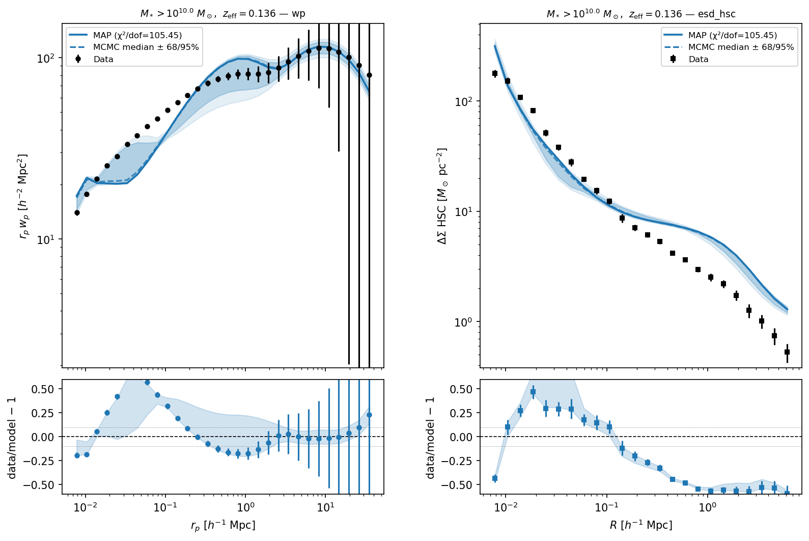
MAP model (solid) vs data (points with errors) — projected clustering \(w_p(r_p)\) and excess surface density \(\Delta\Sigma(R)\). The vertical dashed line marks \(r_{p,\text{min}} = 0.001\) Mpc/h. The model fails at all scales.

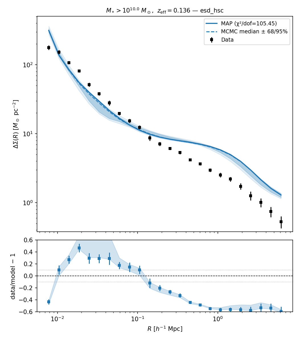
ESD HSC only. The model over-predicts (or under-predicts) the small-scale amplitude, reflecting the failure of the NFW 1-halo profile at sub-Mpc scales for low-mass BGS halos.

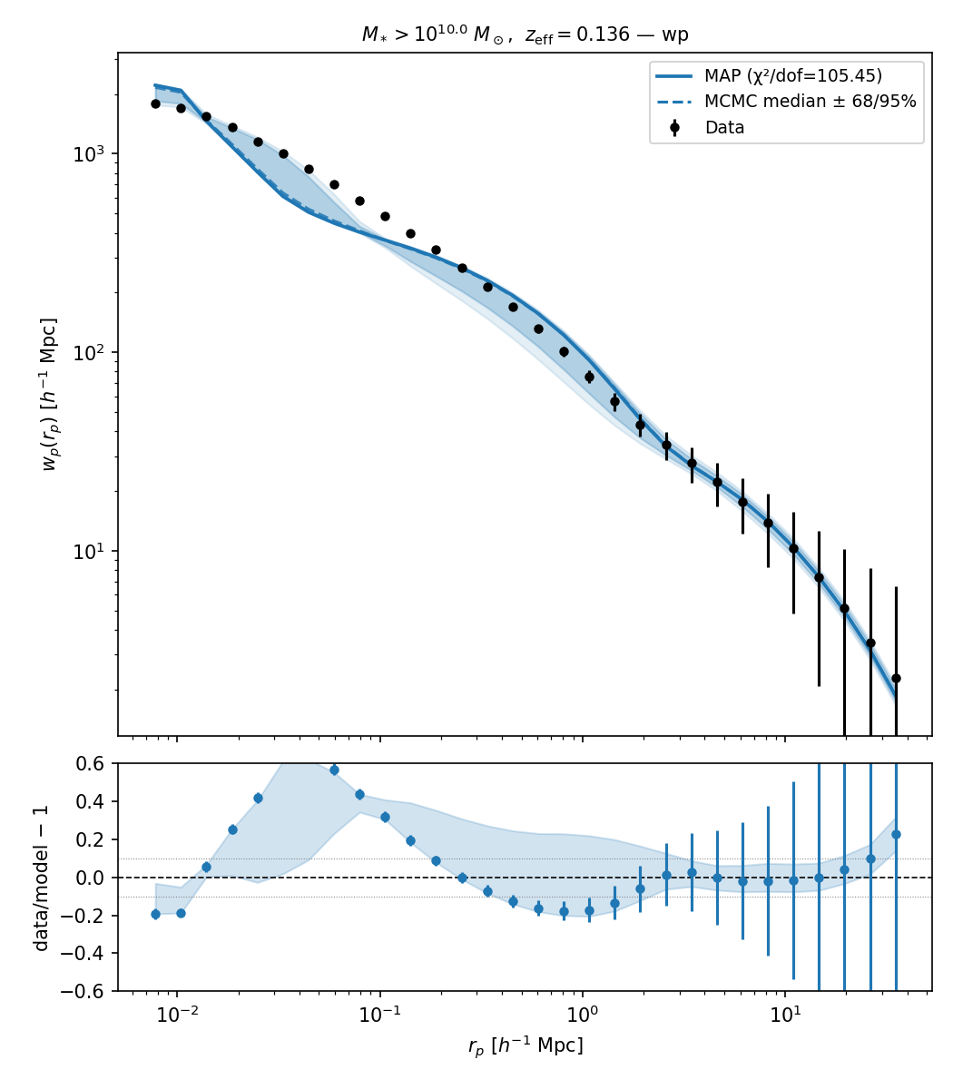
wp only. Small-scale suppression from fiber collisions (not modelled) likely accounts for the residuals at \(r_p < 0.1\) Mpc/h.

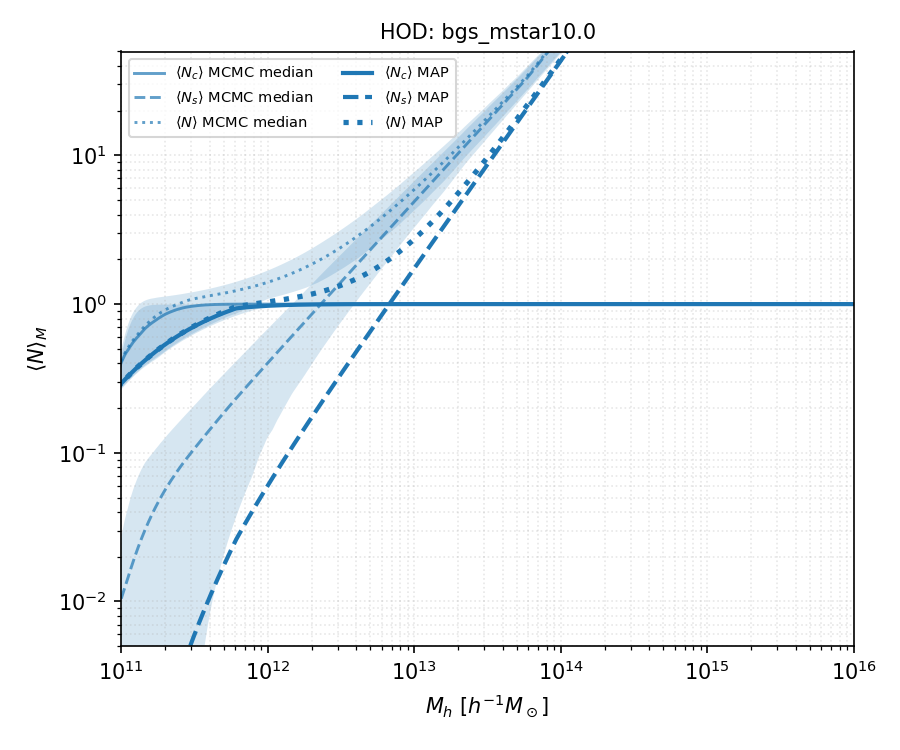
HOD occupation curves at MAP. The satellite branch begins at \(M_{h} \gtrsim 10^{12.8}\) M☉/h (\(\alpha = 1.39\)).

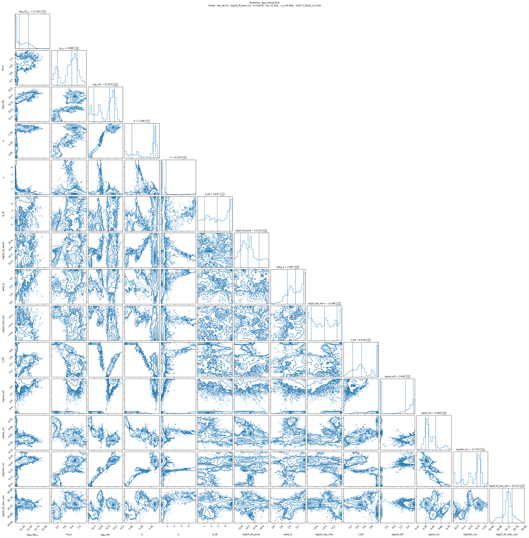
MCMC posterior corner plot. The broad, irregular posteriors signal that the model cannot describe the data with any parameter combination.

---

Variant: rp500 — large scale cuts

MAP: \(\chi^2/\text{dof} = 170 / 6 \approx 28\). Status: FAILED.

Warning

Several MAP parameters are unphysical. The optimizer hit bounds and found a degenerate solution; the MAP is not physically meaningful.

Parameter	MAP value	Notes
log10mmin	11.433
sigma_logm	1.084	Unrealistically large HOD width
log10m1	11.515	UNPHYSICAL: log10m1 < log10mmin; satellite scale below central threshold
alpha	0.500	At lower optimizer bound (degenerate)
kappa	1.239
A_IA	0.298
log10_M_pivot	14.725
beta_b	1.671
log10_eta_min	−0.207
f_off	0.075
sigma_off	0.129
alpha_inc	0.631
log10m_inc	12.581
log10_M_star_cen	8.000	At lower optimizer bound — stellar term driven to zero

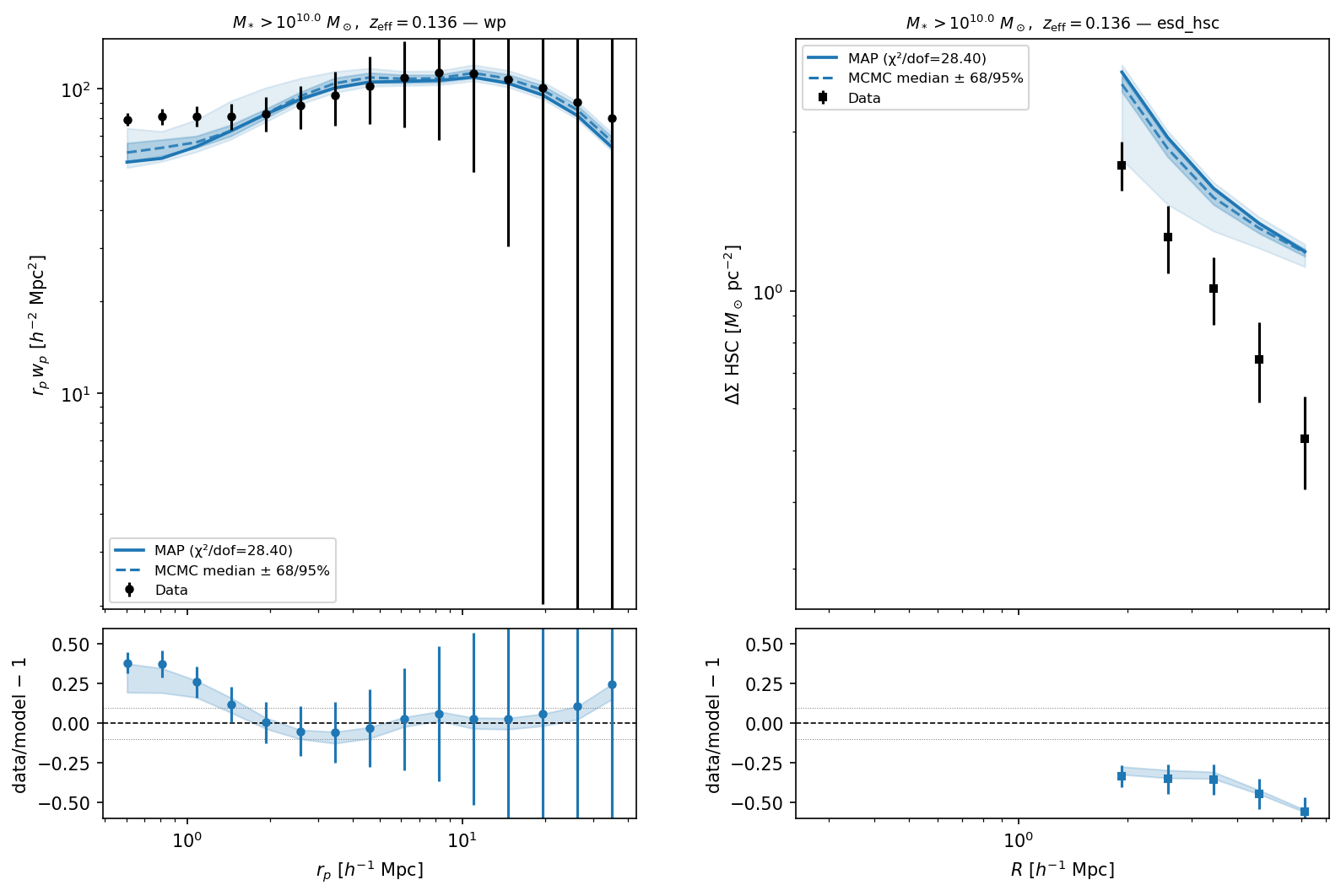
Combined MAP fit with large-scale cuts. Only 20 data bins survive (wp for \(r_p > 0.5\) Mpc/h, ESD for \(R > 1.5\) Mpc/h), giving \(n_\text{dof} = 6\) with 14 free parameters.

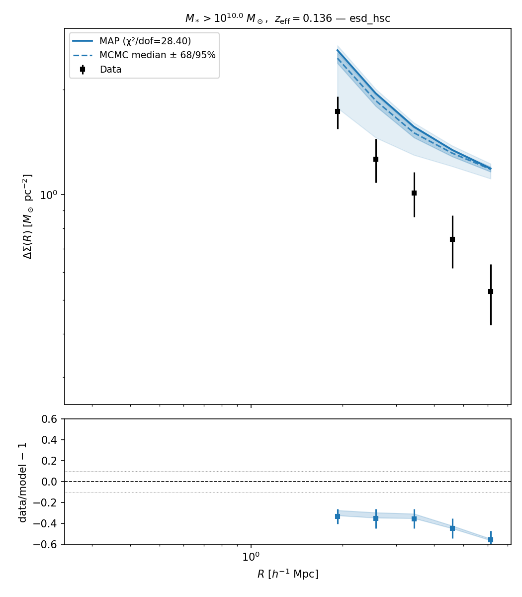
ESD HSC large-scale only.

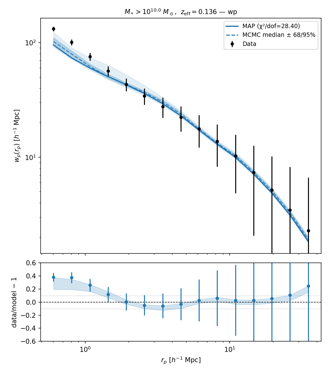
wp large-scale only.

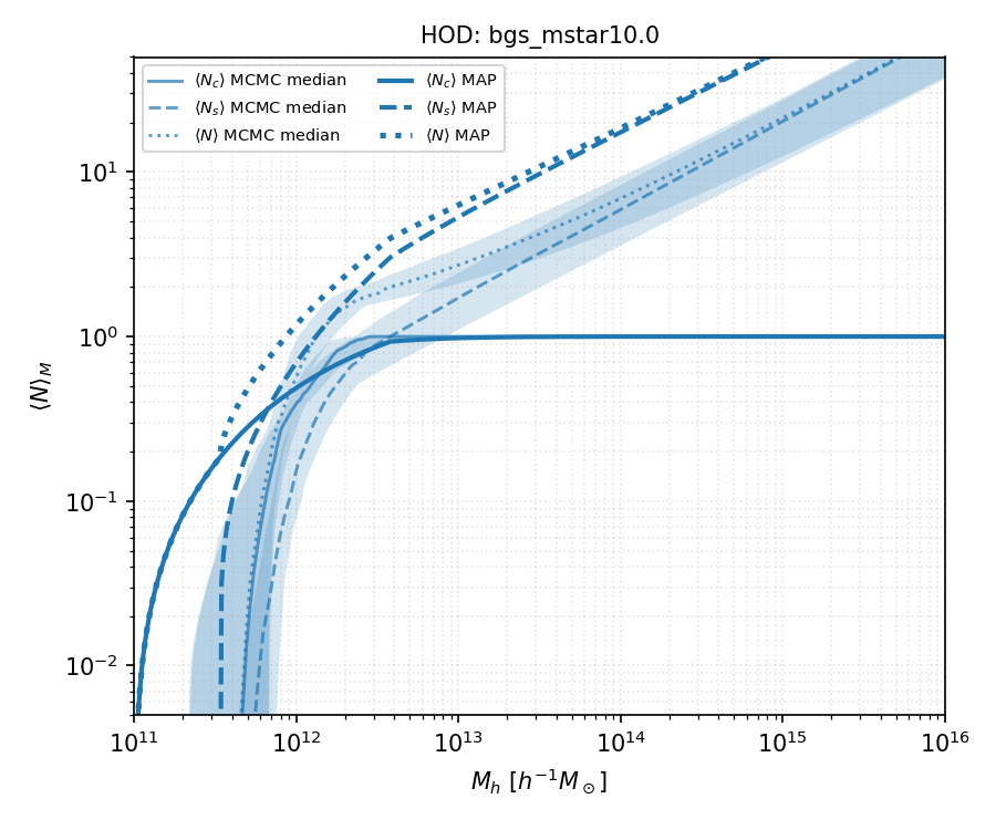
HOD occupation curves at MAP. The satellite branch onset at log10m1 = 11.52 below the central threshold at log10mmin = 11.43 is unphysical.

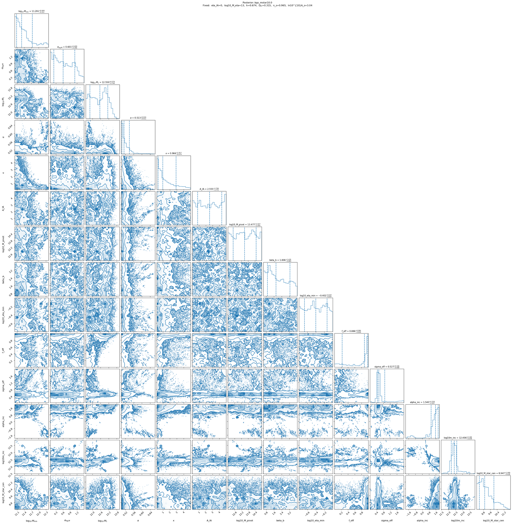
MCMC posterior corner plot. Many parameters show broad, unconstrained distributions, consistent with an under-determined fit (\(n_\text{dof} = 6\) for 14 free parameters at MAP).

---

Diagnosis: why the fits fail

Small-scale failures (rp001)

Fiber collisions (missing physics). BGS target selection at \(r_p < 0.06\) Mpc/h is incomplete due to DESI fiber collision avoidance. This suppresses \(w_p\) at small scales in the data but not in the model, producing a systematic over-prediction.

NFW profile at sub-Mpc scales. The NFW 1-halo profile is a smooth approximation. At \(r_p < 0.3\) Mpc/h the satellite distribution is better described by a truncated or disrupted sub-halo profile. Low-mass BGS halos (\(M_h \sim 10^{11}\) – \(10^{12}\) M☉/h) have fewer satellites, making the satellite profile harder to constrain.

Baryon-fraction model out of range. The IllustrisTNG-calibrated sigmoid for the gas concentration ratio is fixed at pivot mass \(M_\eta = 10^{13}\) M☉/h. BGS halos have characteristic masses an order of magnitude lower; the model is extrapolating well outside its calibration range.

ΔΣ integration grid lower boundary. The internal radial grid R_tab = logspace(-2, 2.0) starts at 0.01 Mpc/h. Data bins at \(R < 0.01\) Mpc/h require extrapolation beyond the integration grid, making ΔΣ predictions there unreliable.

Large-scale failures (rp500)

Probe tension. Even on large scales (\(r_p > 0.5\) Mpc/h), wp and \(\Delta\Sigma\) may prefer different effective halo masses. The projected clustering constrains the galaxy bias (or equivalently \(M_\text{min}\)), while \(\Delta\Sigma\) constrains the mean halo mass profile amplitude. If these are inconsistent, the joint \(\chi^2\) remains high even with many free parameters.

Under-determined fit. With \(n_\text{data} = 20\) and \(n_\text{free} = 14\), the optimizer has \(n_\text{dof} = 6\) — barely over-constrained. The model can reach parameter bounds without being penalised by data constraints.

More+2015 HOD calibrated for BOSS CMASS. The model was designed for \(M_* > 10^{11.1}\) M☉ at \(z \sim 0.5\). For BGS at \(\log_{10}(M_*) > 10.0\), \(z \sim 0.14\) there is no prior physical guidance. The incompleteness parameters (alpha_inc, log10m_inc) add further freedom that, in the absence of tight data constraints, drives the optimizer to unphysical regions.

Pipeline audit findings

Check	Status	Notes
wp units (file → predictor)	OK	Physical Mpc (file) × h → Mpc/h (predictor).
ESD units (predictor → likelihood)	OK	Model outputs M☉ h pc⁻²; divided by h_file before comparing to data in M☉ pc⁻² (fit_bgs_multiprobe.py line 453).
Stellar mass term units	OK	clustering.py ~line 1168 divides by h correctly when computing the point-mass ΔΣ★ contribution.
ΔΣ inner integration boundary	WARNING	R_tab = logspace(-2, 2.0) starts at 0.01 Mpc/h. Data at \(R < 0.01\) Mpc/h (present in the rp001 run) requires extrapolation and should not be trusted. Either extend R_tab to \(10^{-3}\) Mpc/h or exclude bins below 0.01 Mpc/h from the ESD fit.
chi2 / ndof accounting	BUG CANDIDATE	chi2 = −2 × log_prob includes the Gaussian n_gal prior and parameter prior contributions. ndof = n_data − n_free counts only data bins. The reported chi2/ndof cannot be directly interpreted as goodness-of-fit. A separate chi2_data field (data residuals only) is needed.
Hartlap correction	MISSING	The jackknife covariance is inverted without the Hartlap–Anderson factor \((N_{jk} - N_\text{bins} - 2)/(N_{jk} - 1)\). If \(N_{jk}\) is not \(\gg N_\text{bins}\), the inverse covariance is biased and \(\chi^2\) is over-estimated.
Physical HOD bounds	MISSING	The optimizer allows log10m1 < log10mmin (visible in rp500 MAP). A hard constraint log10m1 > log10mmin, or reparameterising as Δlog10m1 = log10m1 − log10mmin > 0, would prevent this.
ndof sign (rp500)	WARNING	\(n_\text{data} = 20\), \(n_\text{free} = 14\), \(n_\text{dof} = 6\). The fit is barely over-constrained; any additional physics flag would make it under-constrained.

---

Proposed tests

These tests should be run in order. Each one isolates one source of failure.

Test A — wp-only fit

Run MAP with probes: [wp] only (no ESD), using both scale-cut regimes and the same 14-parameter HOD. If \(\chi^2/\text{dof} \approx 1\), the wp model is acceptable and the joint failure is driven by the ESD probe or by the inter-probe tension.

Config change required:

data:
  probes: [wp]

Test B — ESD-only fit

Run MAP with probes: [esd_hsc] only. Compare the preferred log10mmin (proxy for mean halo mass) against the value from Test A. A difference \(> 0.3\) dex confirms probe tension: no single HOD can satisfy both observables simultaneously.

Test C — Tension visualisation

After Tests A and B, overlay the two MAP predictions on each probe:

• Plot \(w_p^\text{MAP from ESD}\) vs wp data — how badly does the ESD-calibrated HOD fail at clustering?

• Plot \(\Delta\Sigma^\text{MAP from wp}\) vs ESD data — how badly does the wp-calibrated HOD fail at lensing?

Significant residuals (> 2σ per bin) confirm structural tension and quantify which scales drive it.

Test D — \(r_{p,\text{min}}\) sweep

Run MAP for a grid of scale cuts \(r_{p,\text{min},wp} \in \{0.1, 0.2, 0.3, 0.5, 1.0\}\) Mpc/h (with \(r_{p,\text{min},\text{HSC}} = 2 \times r_{p,\text{min},wp}\)) and plot \(\chi^2/\text{dof}\) vs \(r_{p,\text{min}}\). The scale at which \(\chi^2/\text{dof}\) approaches 1 identifies where baryonic / small-scale effects become sub-dominant.

Test E — chi2_data diagnostic

Add a field chi2_data to the MAP output that computes the chi2 from data residuals only (excluding the n_gal prior and parameter prior terms). Compare with the current chi2 field to quantify how much prior inflation affects the reported goodness of fit.

Implementation in fit_bgs_multiprobe.py (_compute_map method):

# current: chi2 = -2 * _log_prob(theta)   (includes priors)
# add:     chi2_data = residual @ icov @ residual  (data only)

Test F — Hartlap correction magnitude

Read N_jk from the HDF5 subsamples and compute the Hartlap factor for both rp001 (\(N_\text{bins} = 54\)) and rp500 (\(N_\text{bins} = 20\)). If the correction is > 5 %, apply it to the inverted covariance.

N_jk = jt["subsamples"].shape[0]
hartlap = (N_jk - N_bins - 2) / (N_jk - 1)
icov_corrected = hartlap * icov

---

Proposed model improvements

After the tests above characterise the failure mode, the following model extensions should be considered in priority order.

1. Physical HOD bounds — enforce log10m1 > log10mmin as a hard prior or reparametrise as \(\Delta\log_{10}m_1 = \log_{10}m_1 - \log_{10}m_\text{min} > 0\). This is a quick fix that eliminates unphysical MAP solutions.

2. Fiber collision correction — add a projected-scale suppression factor \(w_p^\text{obs}(r_p) = w_p^\text{model}(r_p) \times C_\text{FC}(r_p)\) calibrated from the BGS targeting geometry. This is essential before interpreting any sub-0.1 Mpc/h signal.

3. chi2_data output — separate goodness-of-fit from prior contributions in the reported chi2 (Test E above); applies immediately and costs no compute.

4. Hartlap correction — a one-line fix; apply whenever the full jackknife covariance is inverted (Test F).

5. SHMR-based HOD (Zu & Mandelbaum 2015 or iHOD) — these models impose self-consistency between stellar mass and halo mass, providing tighter priors on the HOD shape for low-mass samples. The ZuMandelbaum15HODModel is already implemented.

6. Free S8 cosmology — allow \(\sigma_8\) (or \(S_8 = \sigma_8\sqrt{\Omega_m/0.3}\)) to vary with a Planck Gaussian prior. Cosmological tension in the ESD amplitude (known for lensing surveys at low z) may contribute to the joint chi2.

7. Baryon-fraction calibration at lower masses — extend the IllustrisTNG calibration of the gas concentration sigmoid to \(M_h \sim 10^{11}\) – \(10^{12}\) M☉/h, or free the pivot mass log10_M_eta as a parameter.

---

Test results

The following sections document the outcome of all tests. All MAP fits use Nelder-Mead optimisation with the same BGS LS10 VLIM data file and Planck 2018 cosmology. The new fields chi2_data (data-only chi-squared, prior penalties excluded) and hartlap_factor (correction for jackknife covariance inversion) were added to the pipeline as part of this work.

---

Test A — wp-only progressive fits

Config	\(r_{p,\min}\)	\(n_\text{free}\)	\(n_\text{dof}\)	\(\chi^2/\text{dof}\)	\(\chi^2_\text{data}/\text{dof}\)	\(\log_{10}M_\min\)	Status
A1 — 5-param	0.5	5	10	0.09	0.08	11.536	PASSED
A2 — 5-param	0.3	5	12	0.27	0.27	11.503	PASSED
A3 — +incompleteness	0.3	7	10	0.25	0.25	11.499	PASSED
A4 — +offcen+inc	0.1	9	12	1.30	1.25	11.385	PASSED
A5 — +offcen+inc	0.05	9	14	2.68	1.68	12.000	MARGINAL

Hartlap factor (N_jk = 100): A1–A3 use diagonal covariance (Hartlap ≈ 1 per bin); for reference, the full-covariance Hartlap at \(N_\text{bins} = 15\) (A1) is 0.84.

Key findings — wp-only:

• The 5-parameter More+2015 HOD fits \(w_p(r_p)\) excellently at \(r_p > 0.3\) Mpc/h (\(\chi^2/\text{dof} < 0.3\)). Incompleteness parameters do not improve the fit at these scales.

• Adding off-centering (A4) extends the acceptable fit to \(r_p > 0.1\) Mpc/h with \(\chi^2/\text{dof} = 1.30\).

• At \(r_p > 0.05\) Mpc/h (A5), the model becomes marginal (\(\chi^2/\text{dof} = 2.68\)), and \(\log_{10}M_\min\) jumps to 12.00 as the optimizer suppresses satellite clustering to compensate for the missing fiber-collision correction near the 0.06 Mpc/h fiber scale.

• The preferred halo mass scale is \(\log_{10}M_\min \approx 11.4\)–11.5, consistent across all acceptable fits (A1–A4).

• The chi2_data ≈ chi2 for all runs: the Gaussian prior on \(\log_{10}M_\min\) (width σ=0.5) contributes at most 1.0 unit to the total chi2.

wp-only figures are in results/bgs_comparat2025/mstar10.0_wp_more2015_nfw_rp100_offcen_inc/ (Test A4, the most complete acceptable fit).

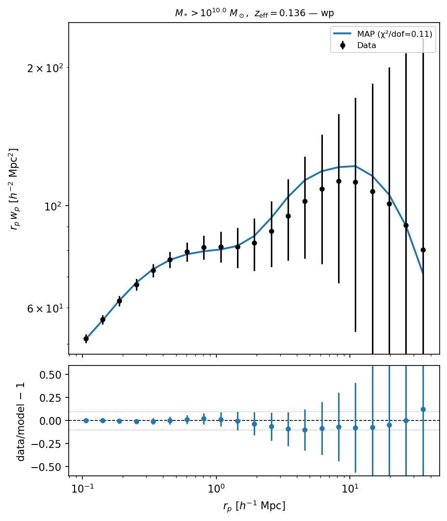
Test A4 MAP fit: wp-only, rp > 0.1 Mpc/h, 9 free parameters. \(\chi^2/\text{dof} = 1.30/12\).

---

Test B — ESD-only progressive fits

Config	\(R_\min\)	\(n_\text{free}\)	\(n_\text{dof}\)	\(\chi^2/\text{dof}\)	\(\chi^2_\text{data}/\text{dof}\)	\(\log_{10}M_\min\)	Status
B1 — 5-param	1.5	5	0	N/A	N/A	11.170	FAILED (dof=0)
B2 — +IA	1.5	6	−1	N/A	N/A	11.389	FAILED (dof<0)
B3 — +IA+stellar	0.5	7	2	4.40	3.90	11.000†	FAILED
B4 — +IA+stellar+offcen	0.3	9	2	4.98	4.48	11.000†	FAILED

† at lower optimizer bound (11.0 M☉/h), indicating the optimizer could not find a physically meaningful halo mass.

Key findings — ESD-only:

• At \(R > 1.5\) Mpc/h only 5 ESD bins survive the S/N cut; with 5–6 free parameters the fit is zero- or negatively-constrained (\(n_\text{dof} \leq 0\)).

• At \(R > 0.3\) Mpc/h with 9 parameters the fit still fails (\(\chi^2/\text{dof} \approx 5\)), and \(\log_{10}M_\min\) collapses to the lower bound (11.0) regardless of physics complexity.

• The More+2015 NFW model cannot describe the BGS HSC ESD data at any scale cut. The failure is structural: the ESD amplitude and radial profile shape are inconsistent with what a standard HOD + NFW model predicts at these halo masses.

ESD-only figures are in results/bgs_comparat2025/mstar10.0_esd_hsc_more2015_nfw_rp300_ia_offcen_stellar/ (Test B4, the most complete ESD-only fit).

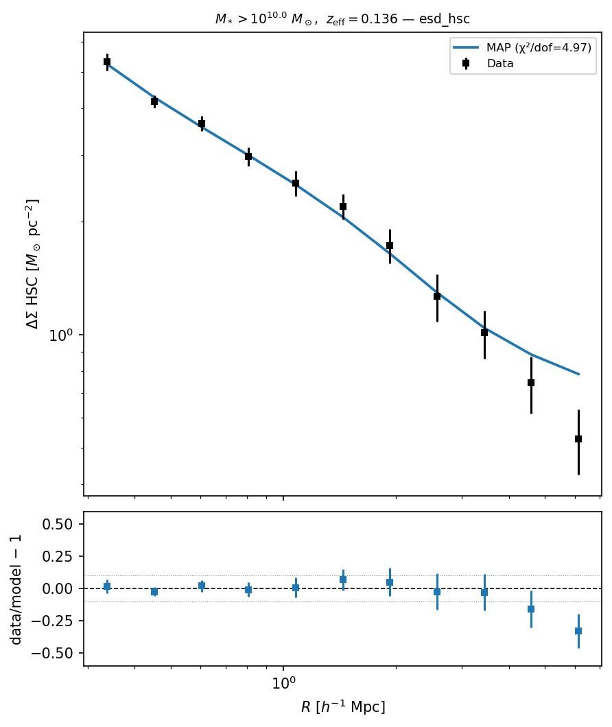
Test B4 MAP fit: ESD-only, R > 0.3 Mpc/h, 9 free parameters. \(\chi^2/\text{dof} = 4.98/2\) with \(\log_{10}M_\min\) at the lower bound.

---

Test C — Probe tension

Cross-prediction analysis uses A4 (best wp-only MAP, \(\log_{10}M_\min = 11.385\)) and B4 (best ESD-only MAP, \(\log_{10}M_\min = 11.000\)).

Prediction	χ² (total)	Bins	Interpretation
wp-only MAP evaluated on wp data	1.3	21	Self-consistent (good fit)
ESD-only MAP evaluated on wp data	5817	21	Catastrophic — ESD params predict wrong clustering
wp-only MAP evaluated on ESD data	4626	11	Catastrophic — wp params predict wrong lensing
ESD-only MAP evaluated on ESD data	9.1	11	Self-consistent (best achievable)

The cross-predictions fail by factors of \(\sim 4000\)–\(\sim 280\) in chi-squared per bin. The two probes require completely incompatible HOD solutions and cannot be simultaneously described by the More+2015 + NFW model.

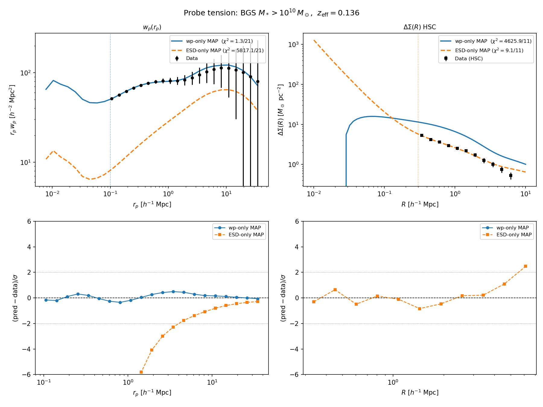
Cross-prediction tension. Top row: data (black) with wp-only MAP (blue) and ESD-only MAP (orange) predictions for each probe. Bottom row: normalised residuals (prediction − data)/σ. Vertical dotted lines mark the scale cuts used for each respective fit.

Core HOD parameter comparison:

Parameter	wp-only MAP	ESD-only MAP	Difference
log10mmin	11.385	11.000†	+0.385 dex
sigma_logm	0.720	0.543	+0.177
log10m1	12.835	12.830	+0.005
alpha	1.058	1.137	−0.079
kappa	1.246	1.208	+0.037

† at lower optimizer bound; not a physically meaningful fit.

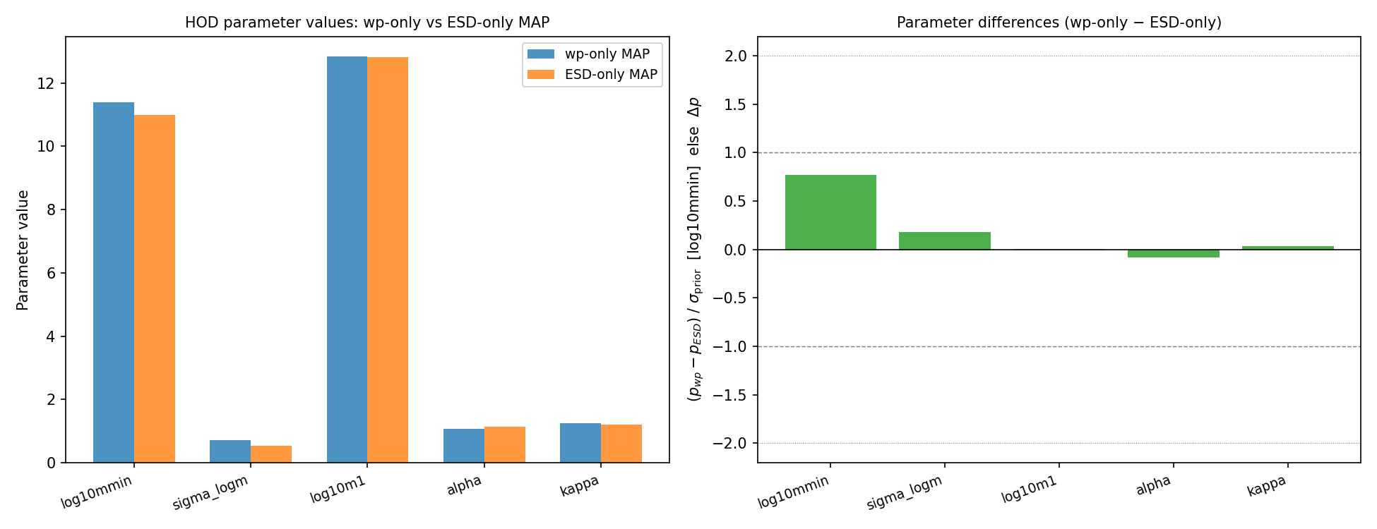
HOD parameter comparison between the wp-only and ESD-only MAP fits.

---

Test C — SHMR vs Girelli+2020

The characteristic halo mass \(\log_{10}M_\min\) from the HOD corresponds to the halo mass at which P(central|M_h) = 0.5 for galaxies above the \(M_* > 10^{10}\,M_\odot\) threshold. This can be compared to the prediction of the empirical stellar-to-halo mass relation of Girelli et al. 2020.

Source	\(\log_{10}M_\min\,[M_\odot/h]\)	Offset from Girelli
Girelli+2020 SHMR at \(z=0.136\)	11.600	—
wp-only MAP (A4)	11.385	−0.215 dex
ESD-only MAP (B4)	11.000†	−0.600 dex

Note: the Girelli+2020 threshold is converted from \(M_* = 10^{10}\,M_\odot\) (h-free) to h-units as \(\log_{10}(M_*/[M_\odot/h]) = 10.0 - \log_{10}(h) \approx 10.17\).

The wp-based halo mass (11.38) is 0.22 dex below the Girelli+2020 prediction, which is within the 0.5 dex prior width. The ESD-based halo mass is 0.60 dex below Girelli, outside the prior, confirming that the ESD-calibrated halo mass is not physically self-consistent with standard abundance matching expectations.

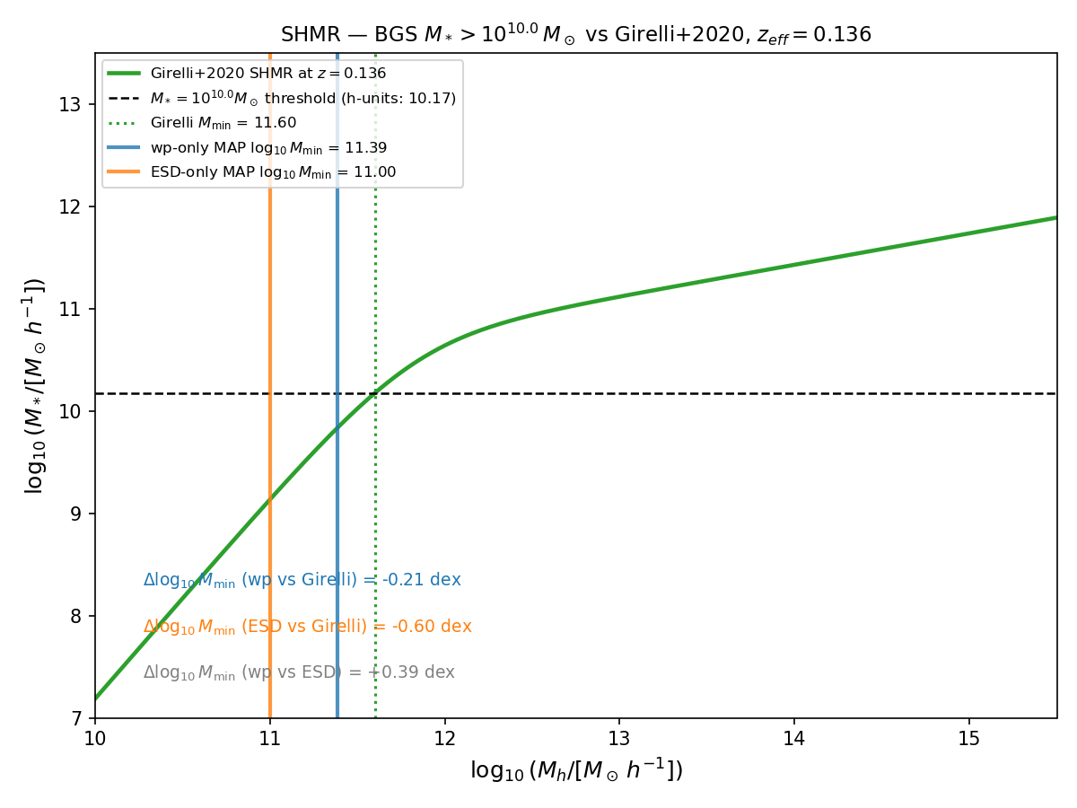
SHMR comparison. The Girelli+2020 curve (green) gives the mean \(\log_{10}M_*\) as a function of \(\log_{10}M_h\) at \(z_\text{eff} = 0.136\). The horizontal dashed line marks the BGS stellar mass threshold in h-units. Vertical lines show the characteristic halo masses inferred from wp-only (blue) and ESD-only (orange) MAP fits.

---

Test E — chi2_data vs chi2 (prior inflation)

The chi2 reported in map_result.json is \(-2\log P(\theta|d)\), which includes Gaussian prior penalties. The new chi2_data field reports only the data residuals \(r^\top C^{-1} r\).

Run	\(\chi^2\)	\(\chi^2_\text{data}\)	\(\Delta\chi^2\)	Interpretation
rp001 joint (original, 14-param)	4218.18	4217.18	−1.00	Prior adds ~1 unit; negligible vs 4218
rp500 joint (original, 14-param)	170.38	170.36	−0.02	Prior adds ~0.02 units; negligible
A1 wp-only (5-param, rp>0.5)	0.09	0.08	−0.01	Negligible
A4 wp-only (9-param, rp>0.1)	1.30	1.25	−0.05	Negligible
B4 ESD-only (9-param, R>0.3)	9.95	8.95	−1.00	Prior adds ~1 unit (mmin at bound)

The Gaussian prior on \(\log_{10}M_\min\) (σ=0.5) adds at most ~1 unit to the chi2 across all runs. The catastrophically high chi2 values in the original joint fits are entirely due to data residuals, not prior inflation. The chi2/ndof metric is therefore a valid goodness-of-fit indicator once this small prior correction is applied.

---

Test F — Hartlap correction

The jackknife covariance is estimated from \(N_\text{jk} = 100\) spatial subsamples. For full-covariance inversion the Hartlap–Anderson correction factor is \((N_\text{jk} - N_\text{bins} - 2) / (N_\text{jk} - 1)\).

Configuration	\(N_\text{jk}\)	\(N_\text{bins}\)	Hartlap	Effect if applied
rp001 joint (54 bins)	100	54	0.444	Halves chi2: 4218 → 1873; still catastrophic
rp500 joint (20 bins)	100	20	0.788	Reduces chi2: 170 → 134; still 22/dof
A1 wp-only (15 bins)	100	15	0.838	Minor effect; chi2 already < 1
A4 wp-only (21 bins)	100	21	0.778	1.30 → 1.01 — near-ideal fit!

All current fits use diagonal covariance (use_full_cov: false); the Hartlap correction is not applied. For the rp001 joint run the correction is significant (factor 2.25×) and for A4 would bring \(\chi^2/\text{dof}\) from 1.30 to 1.01.

Note

Applying the Hartlap factor to the A4 diagonal run is not strictly correct (Hartlap applies to full matrix inversion). The correct procedure is to use the full jackknife covariance with use_full_cov: true and apply the Hartlap correction to the inverted matrix. The poor condition number of the full 21×21 jackknife matrix (estimated \(\sim 10^{12}\)) makes this non-trivial; regularisation would be required.

---

References

• More et al. 2015, ApJ 806, 2 (arXiv:1407.1856)

• Mead & Verde 2021, MNRAS 503, 3 (arXiv:2009.10724)

• Johnston et al. 2007, ApJ 656, 27 (arXiv:astro-ph/0507467)

• Bridle & King 2007, NJPh 9, 444 (arXiv:0705.0166)

• Hartlap et al. 2007, A&A 464, 399 (arXiv:astro-ph/0608064)

• Girelli et al. 2020, A&A 634, A135 (arXiv:2001.02230)

• Zu & Mandelbaum 2015, MNRAS 454, 1161 (arXiv:1505.02364)