Stage-IV forecast: expected cosmology from the combined multi-wavelength surveys

This page turns the differentiable gas–galaxy–AGN pipeline into a believable expectation for the cosmological precision reachable at the end of the current (Stage-IV) survey generation, as a function of the small-scale cut. Where the Sensitivity study: differentiable pipeline, scale cuts and degeneracy breaking page uses a constant relative error to expose the information and degeneracy structure, this page assigns realistic, per-observable, scale-dependent Gaussian errors matched to the surveys that will actually measure each map, and reports $\sigma(\Omega_m,\sigma_8,S_8)$ and the $(\Omega_m,\sigma_8)$ figure of merit.

The survey list and the observable-to-survey mapping follow the multi-wavelength “by 2030” programme laid out in the 2026 HDR (Comparat): galaxy maps from Rubin/LSST (photometry) and DESI+4MOST (spectroscopy), weak lensing from Euclid+Roman, thermal SZ from Planck/ACT/SPT, soft X-rays from eROSITA, and AGN from X-ray to radio — jointly modelled through their auto- and cross-correlations without a scale cut.

Code: hod_mod.scripts.forecasts.run_stage4_forecast.

The survey combination and the observables 

The twelve observables of the pipeline map onto the Stage-IV facilities as follows. Sky areas are from the HDR survey table (Rubin/LSST $\sim18\,000$ deg², $r\approx27.5$ at 10-yr depth; Euclid $15\,000$ deg²; DESI $\sim14\,000$ deg², $\sim35$M galaxies/QSOs, with 4MOST completing the South; Roman wide IR from 2027; ACT $12\,000$ deg², SPT-3G $\sim1\,500$ deg², Planck full sky; eROSITA all-sky soft X-ray, $f_{\rm sky}\approx0.35$ German extragalactic footprint); the effective sky fraction $f_{\rm sky}$ is the overlap relevant to each statistic.

Observable → Stage-IV survey mapping (effective $f_{\rm sky}$ used).
Observable	Survey(s)	$f_{\rm sky}$
$w_p(r_p)$	DESI + 4MOST (spectroscopic clustering)	0.35
$\Delta\Sigma(R)$	LSST / Euclid / Roman shapes × DESI / LSST lenses (galaxy–galaxy lensing)	0.25
$C_\ell^{\kappa\kappa}$	LSST + Euclid + Roman (cosmic shear)	0.40
$C_\ell^{gy}$	DESI / LSST × ACT / SPT / Planck (thermal SZ)	0.30
$C_\ell^{gX}$	DESI / LSST × eROSITA soft X-ray (0.5–2 keV)	0.35
$C_\ell^{XX}$	eROSITA soft X-ray auto	0.35
$\Phi(L_X)$	eROSITA AGN X-ray luminosity function	0.35
$C_\ell^{\kappa_c\kappa_c}, C_\ell^{g\kappa_c}, C_\ell^{\kappa\kappa_c}$	ACT / SPT / Planck CMB lensing (auto and × galaxies / shear)	0.35–0.40
$n_{\rm gal}, \Phi(M_*)$	DESI / LSST galaxy number density and stellar-mass function	0.35

The error model 

Each data point carries a diagonal Gaussian error $\sigma_i$ with a cosmic variance floor set by $f_{\rm sky}$ (grounded in the survey areas) plus a noise-to-signal term that grows towards small scales (shot / shape / instrument / background):

Angular spectra ($C_\ell^{gX},C_\ell^{gy},C_\ell^{XX},C_\ell^{\kappa\kappa}$) — the Knox formula per (log-)$\ell$ bin

\[\frac{\Delta C_\ell}{C_\ell} = \sqrt{\frac{2}{N_{\rm modes}(\ell)}} \left(1 + \frac{N_\ell}{C_\ell}\right),\quad N_{\rm modes}=(2\ell+1)\,\ell\,\Delta\ln\ell\,f_{\rm sky},\quad \frac{N_\ell}{C_\ell}=r_N\Big(\frac{\ell}{100}\Big)^{a_N}.\]
Projected $w_p,\Delta\Sigma$ — $\sigma/d=\sqrt{(f_{\rm CV}/\sqrt{f_{\rm sky}})^2 + (r_N\,(1\,{\rm Mpc}/h/r_p)^{a_N})^2}$ (cosmic-variance floor $f_{\rm CV}=0.3\%$ + shot/shape noise rising to small $r_p$). The floor is set well below a percent because a Stage-IV projected measurement spans a multi-${\rm Gpc}^3$ volume and averages over a huge number of independent large-scale modes, so the irreducible sample variance per $r_p$ bin is small; at $f_{\rm sky}=0.35$ this floor is $\approx0.5\%$.
XLF $\Phi(L_X)$ — a constant Poisson-like per-dex error.

The noise-to-signal parameters $(r_N,a_N)$ are effective per-bin values for the end-of-survey Stage-IV depth: they are anchored on the current measurement signal-to-noise (e.g. the Comparat et al. 2025 eROSITA galaxy–X-ray cross-correlation, which measures the $L_X$–$M$ slope to $\alpha_{\rm SR}=1.63\pm0.09$) and standard shape / shot budgets, but scaled to the Stage-IV source and tracer densities — so the noise-to-signal at the pivot and its small-scale growth $a_N$ are markedly milder than a Stage-III forecast (higher $n_{\rm eff}$ pushes the shot/shape-noise crossover to smaller scales). They are explicit, tabulated assumptions — the honest choice, rather than a false-precision analytic covariance built on many un-published numbers:

Per-observable Stage-IV error parameters.
Observable	$f_{\rm sky}$	$r_N$	$a_N$	Prescription
$w_p$	0.35	0.015	0.5	floor + noise (projected)
$\Delta\Sigma$	0.25	0.03	0.6	floor + noise (shape-noise limited)
$C_\ell^{\kappa\kappa}$	0.40	0.05	1.1	Knox (shape noise)
$C_\ell^{gy}$	0.30	0.25	0.9	Knox (tSZ noise/beam)
$C_\ell^{gX}$	0.35	0.30	1.0	Knox (X-ray background/shot)
$C_\ell^{XX}$	0.35	0.70	1.2	Knox (X-ray auto, noisiest)
$\Phi(L_X)$	0.35	0.05	—	Poisson (constant per dex)
$C_\ell^{\kappa_c\kappa_c}$	0.40	0.25	0.9	Knox (CMB-lensing reconstruction)
$C_\ell^{g\kappa_c}$	0.35	0.15	0.7	Knox (galaxy × CMB lensing)
$C_\ell^{\kappa\kappa_c}$	0.35	0.20	0.9	Knox (shear × CMB lensing)
$n_{\rm gal}$	0.35	0.01	—	number density (1 %)
$\Phi(M_*)$	0.35	0.03	—	per-dex (3 %)

The resulting per-bin errors (left panel of the figure below) fall to sub-percent on the best-sampled projected and mid-$\ell$ scales, and rise to tens of percent both in the lowest-$\ell$ (few-mode, cosmic-variance-limited) bins and for the noise-dominated X-ray auto $C_\ell^{XX}$ — milder throughout than a Stage-III forecast.

Expected constraints as a function of scale cut 

Marginalising over the full 31-parameter vector (5 cosmological — $\Omega_m,\sigma_8,h,n_s,\Omega_b$ with $h,n_s,\Omega_b$ carrying Planck/BBN priors — 9 HOD, 6 X-ray gas, 2 baryon-feedback, $\beta_P$, $\log_{10}\rm DC$, 7 Powell AGN — see the Sensitivity study: differentiable pipeline, scale cuts and degeneracy breaking parameter inventory) with weakly-informative nuisance priors, and propagating to $S_8=\sigma_8(\Omega_m/0.3)^{1/2}$:

Expected $1\sigma$ from the combined Stage-IV data vector (all twelve maps), LSS-only, and adding a Planck prior on $(\Omega_m,\sigma_8)$. Percentages are relative to the fiducial ($\Omega_m=0.31,\ \sigma_8=0.811,\ S_8=0.825$).
$R_{\min}$ [Mpc/h]	$\sigma(\Omega_m)$	$\sigma(\sigma_8)$	$\sigma(S_8)$	FoM	$\sigma(S_8)$ +Planck
0.1	$1.2\times10^{-3}$ (0.38 %)	$1.5\times10^{-3}$ (0.19 %)	$1.3\times10^{-3}$ (0.15 %)	$7.4\times10^{5}$	$1.3\times10^{-3}$ (0.15 %)
0.5	$1.7\times10^{-3}$ (0.53 %)	$2.6\times10^{-3}$ (0.32 %)	$1.5\times10^{-3}$ (0.18 %)	$4.2\times10^{5}$	$1.4\times10^{-3}$ (0.17 %)
2.5	$2.3\times10^{-3}$ (0.74 %)	$4.6\times10^{-3}$ (0.56 %)	$2.7\times10^{-3}$ (0.33 %)	$1.7\times10^{5}$	$2.4\times10^{-3}$ (0.29 %)
5.0	$2.5\times10^{-3}$ (0.80 %)	$6.4\times10^{-3}$ (0.78 %)	$4.6\times10^{-3}$ (0.56 %)	$9.4\times10^{4}$	$3.5\times10^{-3}$ (0.43 %)
10.0	$2.6\times10^{-3}$ (0.84 %)	$8.8\times10^{-3}$ (1.08 %)	$7.1\times10^{-3}$ (0.86 %)	$5.8\times10^{4}$	$4.5\times10^{-3}$ (0.55 %)

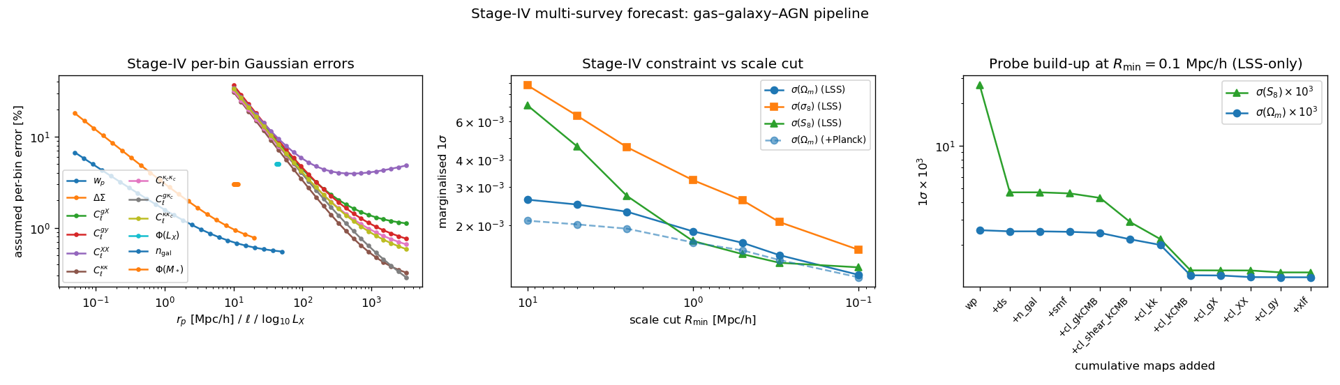
_images/stage4_forecast.png — *Left:* the assumed Stage-IV per-bin fractional errors for each map — sub-percent on the best-sampled scales, rising to tens of percent in the lowest-$\ell$ (few-mode) bins and for the X-ray auto. *Middle:* the marginalised $\sigma(\Omega_m),\sigma(\sigma_8),\sigma(S_8)$ versus scale cut (LSS-only; dashed = adding a Planck prior). *Right:* the cumulative build-up of $\sigma(\Omega_m)$ and $\sigma(S_8)$ as each map is added, at $R_{\min}=0.1$ Mpc/h, grouped clustering ($w_p,\Delta\Sigma$) → abundances ($n_{\rm gal},\Phi(M_*)$) → lensing / CMB-lensing → X-ray and SZ.

Reading the forecast:

Expected precision. The full combination reaches $\sigma(S_8)\approx0.15\%$, $\sigma(\sigma_8)\approx0.19\%$, $\sigma(\Omega_m)\approx0.38\%$ at $R_{\min}=0.1$ Mpc/h — an order of magnitude below current large-scale-structure results (DESI DR1 full-shape $\sim3.2/4/4\%$ on $\Omega_m/\sigma_8/S_8$; DES-Y6 3×2pt $7.1/4.3/1.4\%$; KiDS-Legacy shear $1.8\%$ on $\Sigma_8$) and tighter than the CMB ($\sigma_8$ $0.5\%$, $\Omega_m$ $1.6\%$). This is the quantitative version of the HDR statement that full-shape + 3×2pt constraints “will rival CMB results.”
The scale cut is worth a factor of a few. Pushing $R_{\min}$ from 10 to 0.1 Mpc/h tightens $\sigma(S_8)$ by $\sim5.6\times$ and $\sigma(\Omega_m)$ by $\sim2.2\times$ — the payoff of a model that can be trusted below $\sim$ Mpc scales, which is the whole motivation for the gas/AGN feedback modelling.
The lensing sector drives $S_8$, but the clustering + gas probes make it safe. The right panel’s cumulative build-up (at $R_{\min}=0.1$ Mpc/h, in the order clustering → abundances → lensing → X-ray/SZ) shows $w_p$ alone reaches only $\sigma(S_8)\approx3.2\%$; adding galaxy–galaxy lensing ($\Delta\Sigma$) collapses it to $\sim0.57\%$; the abundances ($n_{\rm gal},\Phi(M_*)$) are essentially flat; the lensing sector — galaxy×CMB-lensing, shear×CMB-lensing, cosmic shear and the CMB-lensing auto — drives the decisive drop to $\sim0.16\%$ (the CMB-lensing auto alone taking $0.27\to0.16\%$); and the X-ray / tSZ / XLF legs tighten it only marginally further (to $0.15\%$) but calibrate the baryon systematic. The value of the X-ray/SZ legs is not raw $S_8$ signal but the de-biasing of the lensing (the baryon calibration quantified on the Sensitivity study: differentiable pipeline, scale cuts and degeneracy breaking page).
Adding a Planck prior helps most where the LSS data are weakest (large scale cuts): at $R_{\min}=10$ Mpc/h it tightens $\sigma(S_8)$ by $\sim1.6\times$, but at $R_{\min}=0.1$ Mpc/h the LSS combination is already within $\sim1\%$ of the joint result — i.e. the small-scale multi-wavelength data are self-sufficient.
The AGN XLF adds negligibly here because the AGN accretion sector is marginalised (its cosmological amplitude is degenerate with the active fraction); with the accretion sector externally pinned it contributes at the $\times1.03\text{–}1.1$ level in $\sigma(\Omega_m)$ (--agn-pinned; see the Sensitivity study: differentiable pipeline, scale cuts and degeneracy breaking XLF section).

Robustness to the baryon-fraction model: a galaxy×tSZ test 

The forecast fixes the hot-gas fraction $f_b(M)$ to the monotonic BaryonFractionSigmoid. Is that modelling choice quietly driving the cosmology? To check, we swap in the physically-motivated non-monotonic BaryonFractionUpturn — a double sigmoid with the same group-scale suppression plus a low-mass upturn, where AGN feedback is weak in dwarf halos and the cold CGM gas fraction rises again (EAGLE / IllustrisTNG / FLAMINGO; Zhang et al. 2025). The free group pivot $\log_{10}M_{\rm pivot}$ is reused as the upturn’s $M_{\rm hi}$, so the 31-parameter vector is identical and only the $f_b(M)$ shape changes (ForwardModel(baryon_model="upturn")). The two shapes diverge only below $\sim10^{13}\,M_\odot/h$: the upturn fills in the group-scale valley, making $f_b$ about $1.4\text{–}1.5\times$ higher at $10^{12}\text{–}10^{13.5}$ — exactly the halos that host the $M_*>10$ galaxies.

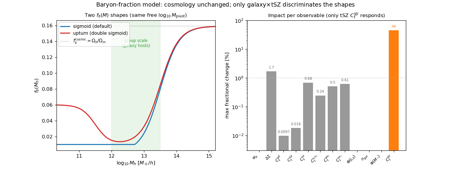
_images/stage4_baryon_model.png — *Left:* the two baryon-fraction shapes at the fiducial (they agree at cluster scales, where both recover $f_b^{\rm cosmic}$, and in the deep valley, but the upturn lifts $f_b$ at group and dwarf masses). *Right:* the maximum fractional change this induces in each fiducial observable — **only the thermal SZ** $C_\ell^{gy}$ **responds** ($\sim40\%$); every other statistic moves by $<2\%$.

Two results follow. First, the cosmological constraints are unchanged:

Stage-IV $1\sigma$ (LSS-only) under the two baryon-fraction shapes.
$R_{\min}$ [Mpc/h]	$f_b$ model	$\sigma(\Omega_m)$	$\sigma(\sigma_8)$	$\sigma(S_8)$
0.1	sigmoid	$1.18\times10^{-3}$	$1.54\times10^{-3}$	$1.28\times10^{-3}$
0.1	upturn	$1.17\times10^{-3}$	$1.54\times10^{-3}$	$1.24\times10^{-3}$
2.5	sigmoid	$2.30\times10^{-3}$	$4.56\times10^{-3}$	$2.72\times10^{-3}$
2.5	upturn	$2.32\times10^{-3}$	$4.57\times10^{-3}$	$2.65\times10^{-3}$

The differences are $\le3\%$ ($\sigma(S_8)$ is marginally tighter with the upturn) — within the modelling noise. The reason the constraints do not move even though $C_\ell^{gy}$ shifts by 40 % is that the Fisher information depends on the shape of $\partial\ln O/\partial\theta$: the 40 % is a pure amplitude that is degenerate with the gas/pressure nuisances ($\beta_P,\log_{10}M_{\rm pivot}$) and marginalises away at no cosmological cost.

Second, and more useful, the test shows which observable actually carries the group-scale baryon content. The thermal SZ pressure scales as $f_b$ (linear, with a shallow mass weighting), so $C_\ell^{gy}$ sees the group gas directly and changes by $\sim40\%$. The X-ray, by contrast, scales as $f_b^2$ with a steep $L_X$–$M$ slope, so $C_\ell^{gX}$/$C_\ell^{XX}$ are dominated by massive clusters (where both models recover $f_b^{\rm cosmic}$) and are blind ($0.01\%$); clustering (satellites trace the dark matter) and the abundances do not depend on $f_b$ at all. The whole galaxy–galaxy and CMB-lensing sector moves by $<1\%$.

The conclusion mirrors the parameter inventory: whether $f_b$ turns up again at low mass is a modelling / systematics question that the galaxy×tSZ cross-correlation can settle decisively (a $\sim40\%$ signal), not one that degrades the cosmological error bars once the feedback sector is marginalised. Freeing the upturn amplitude $f_b^{\rm lo,amp}$ as a genuine extra parameter would add a nuisance direction that $C_\ell^{gy}$ — and only $C_\ell^{gy}$ — constrains.

Caveats 

These are forecasts under stated assumptions, to be read as expected orders of magnitude, not guarantees. The table above uses a diagonal Gaussian error model: it neglects most of the cross-observable covariance (which correlates the maps that trace the same field and would loosen the joint constraint somewhat) and the non-Gaussian small-scale covariance. An analytic Gaussian covariance with cross-observable correlations — exact for the lensing triplet $\{C_\ell^{\kappa\kappa},C_\ell^{\kappa\kappa_c},C_\ell^{\kappa_c\kappa_c}\}$ — is available (hod_mod.forecast.covariance, --covariance gaussian) and is the next increment. A single effective redshift is used (no tomography), the cosmology is LCDM through the Eisenstein–Hu $P(k)$ (no $w_0w_a$ / $\sum m_\nu$ yet), and the X-ray/tSZ legs use analytic differentiable surrogates. Removing each of these approximations is the subject of the staged plan on the Sensitivity study: differentiable pipeline, scale cuts and degeneracy breaking page (couple the real AGN into the cross-spectra; add $n_{\rm gal}$, RSD, $C_\ell^{yy}$, CMB-lensing crosses and AGN clustering; go tomographic; swap in a $w_0w_a\nu$ emulator for $P(k)$).

Reproducing this forecast 

JAX_PLATFORMS=cpu HOD_MOD_RESULTS=/path/to/results \
  python -m hod_mod.scripts.forecasts.run_stage4_forecast \
    --rmin 0.1 0.3 0.5 1 2.5 5 10           # add --agn-pinned for the XLF-unlocked case

Outputs ($HOD_MOD_RESULTS/stage4_forecast/): stage4_forecast.json (the full table + error model), stage4_forecast.npz (Jacobian, per-bin errors, row metadata) and stage4_forecast.png (also copied into docs/_images/).

\(R_{\min}\) [Mpc/h]	\(\sigma(\Omega_m)\)	\(\sigma(\sigma_8)\)	\(\sigma(S_8)\)	FoM	\(\sigma(S_8)\) +Planck
0.1	\(1.2\times10^{-3}\) (0.38 %)	\(1.5\times10^{-3}\) (0.19 %)	\(1.3\times10^{-3}\) (0.15 %)	\(7.4\times10^{5}\)	\(1.3\times10^{-3}\) (0.15 %)
0.5	\(1.7\times10^{-3}\) (0.53 %)	\(2.6\times10^{-3}\) (0.32 %)	\(1.5\times10^{-3}\) (0.18 %)	\(4.2\times10^{5}\)	\(1.4\times10^{-3}\) (0.17 %)
2.5	\(2.3\times10^{-3}\) (0.74 %)	\(4.6\times10^{-3}\) (0.56 %)	\(2.7\times10^{-3}\) (0.33 %)	\(1.7\times10^{5}\)	\(2.4\times10^{-3}\) (0.29 %)
5.0	\(2.5\times10^{-3}\) (0.80 %)	\(6.4\times10^{-3}\) (0.78 %)	\(4.6\times10^{-3}\) (0.56 %)	\(9.4\times10^{4}\)	\(3.5\times10^{-3}\) (0.43 %)
10.0	\(2.6\times10^{-3}\) (0.84 %)	\(8.8\times10^{-3}\) (1.08 %)	\(7.1\times10^{-3}\) (0.86 %)	\(5.8\times10^{4}\)	\(4.5\times10^{-3}\) (0.55 %)

\(R_{\min}\) [Mpc/h]	\(f_b\) model	\(\sigma(\Omega_m)\)	\(\sigma(\sigma_8)\)	\(\sigma(S_8)\)
0.1	sigmoid	\(1.18\times10^{-3}\)	\(1.54\times10^{-3}\)	\(1.28\times10^{-3}\)
0.1	upturn	\(1.17\times10^{-3}\)	\(1.54\times10^{-3}\)	\(1.24\times10^{-3}\)
2.5	sigmoid	\(2.30\times10^{-3}\)	\(4.56\times10^{-3}\)	\(2.72\times10^{-3}\)
2.5	upturn	\(2.32\times10^{-3}\)	\(4.57\times10^{-3}\)	\(2.65\times10^{-3}\)

Stage-IV forecast: expected cosmology from the combined multi-wavelength surveys

The survey combination and the observables

The error model

Expected constraints as a function of scale cut

Robustness to the baryon-fraction model: a galaxy×tSZ test

Caveats

Reproducing this forecast